
Path attribution methods are a gradient-based way
of explaining deep models. These methods require choosing a
hyperparameter known as the baseline input.
What does this hyperparameter mean, and how important is it? In this article,
we investigate these questions using image classification networks
as a case study. We discuss several different ways to choose a baseline
input and the assumptions that are implicit in each baseline.
Although we focus here on path attribution methods, our discussion of baselines
is closely connected with the concept of missingness in the feature space –
a concept that is critical to interpretability research.
Introduction
If you are in the business of training neural networks,
you might have heard of the integrated gradients method, which
was introduced at
ICML two years ago
The method computes which features are important
to a neural network when making a prediction on a
particular data point. This helps users
understand which features their network relies on.
Since its introduction,
integrated gradients has been used to interpret
networks trained on a variety of data types,
including retinal fundus images
and electrocardiogram recordings
If you’ve ever used integrated gradients,
you know that you need to define a baseline input (x’) before
using the method. Although the original paper discusses the need for a baseline
and even proposes several different baselines for image data – including
the constant black image and an image of random noise – there is
little existing research about the impact of this baseline.
Is integrated gradients sensitive to the
hyperparameter choice? Why is the constant black image
a “natural baseline” for image data? Are there any alternative choices?
In this article, we will delve into how this hyperparameter choice arises,
and why understanding it is important when you are doing model interpretation.
As a case-study, we will focus on image classification models in order
to visualize the effects of the baseline input. We will explore several
notions of missingness, including both constant baselines and baselines
defined by distributions. Finally, we will discuss different ways to compare
baseline choices and talk about why quantitative evaluation
remains a difficult problem.
Image Classification
We focus on image classification as a task, as it will allow us to visually
plot integrated gradients attributions, and compare them with our intuition
about which pixels we think should be important. We use the Inception V4 architecture
neural network designed for the ImageNet dataset
in which the task is to determine which class an image belongs to out of 1000 classes.
On the ImageNet validation set, Inception V4 has a top-1 accuracy of over 80%.
We download weights from TensorFlow-Slim
and visualize the predictions of the network on four different images from the
validation set.
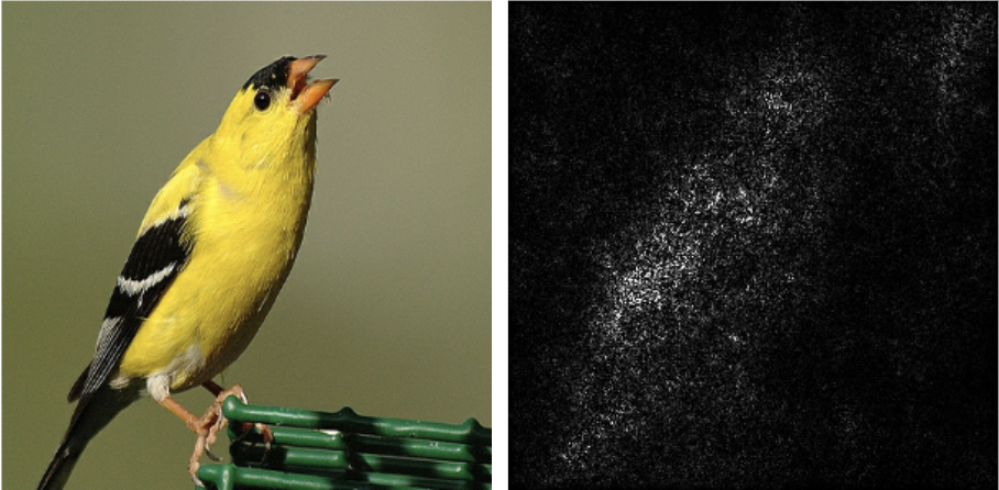
network correctly classifies all images with high confidence.
Left: Pixel-wise attributions of the Inception V4 network using integrated gradients.
You might notice that some attributions highlight pixels that do not seem important
relative to the true class label.
Although state of the art models perform well on unseen data,
users may still be left wondering: how did the model figure
out which object was in the image? There are a myriad of methods to
interpret machine learning models, including methods to
visualize and understand how the network represents inputs internally
feature attribution methods that assign an importance score to each feature
for a specific input
and saliency methods that aim to highlight which regions of an image
the model was looking at when making a decision
These categories are not mutually exclusive: for example, an attribution method can be
visualized as a saliency method, and a saliency method can assign importance
scores to each individual pixel. In this article, we will focus
on the feature attribution method integrated gradients.
Formally, given a target input (x) and a network function (f),
feature attribution methods assign an importance score (phi_i(f, x))
to the (i)th feature value representing how much that feature
adds or subtracts from the network output. A large positive or negative (phi_i(f, x))
indicates that feature strongly increases or decreases the network output
(f(x)) respectively, while an importance score close to zero indicates that
the feature in question did not influence (f(x)).
In the same figure above, we visualize which pixels were most important to the network’s correct
prediction using integrated gradients.
The pixels in white indicate more important pixels. In order to plot
attributions, we follow the same design choices as
That is, we plot the absolute value of the sum of feature attributions
across the channel dimension, and cap feature attributions at the 99th percentile to avoid
high-magnitude attributions dominating the color scheme.
A Better Understanding of Integrated Gradients
As you look through the attribution maps, you might find some of them
unintuitive. Why does the attribution for “goldfinch” highlight the green background?
Why doesn’t the attribution for “killer whale” highlight the black parts of the killer whale?
To better understand this behavior, we need to explore how
we generated feature attributions. Formally, integrated gradients
defines the importance value for the (i)th feature value as follows:
$$phi_i^{IG}(f, x, x’) = overbrace{(x_i – x’_i)}^{text{Difference from baseline}}
times underbrace{int_{alpha = 0}^ 1}_{text{From baseline to input…}}
overbrace{frac{delta f(x’ + alpha (x – x’))}{delta x_i} d alpha}^{text{…accumulate local gradients}}
$$
where (x) is the current input,
(f) is the model function and (x’) is some baseline input that is meant to represent
“absence” of feature input. The subscript (i) is used
to denote indexing into the (i)th feature.
As the formula above states, integrated gradients gets importance scores
by accumulating gradients on images interpolated between the baseline value and the current input.
But why would doing this make sense? Recall that the gradient of
a function represents the direction of maximum increase. The gradient
is telling us which pixels have the steepest local slope with respect
to the output. For this reason, the gradient of a network at the input
was one of the earliest saliency methods.
Unfortunately, there are many problems with using gradients to interpret
deep neural networks
One specific issue is that neural networks are prone to a problem
known as saturation: the gradients of input features may have small magnitudes around a
sample even if the network depends heavily on those features. This can happen
if the network function flattens after those features reach a certain magnitude.
Intuitively, shifting the pixels in an image by a small amount typically
doesn’t change what the network sees in the image. We can illustrate
saturation by plotting the network output at all
images between the baseline (x’) and the current image. The figure
below displays that the network
output for the correct class increases initially, but then quickly flattens.
Notice that the network output saturates the correct class
at small values of (alpha). By the time (alpha = 1),
the network output barely changes.
What we really want to know is how our network got from
predicting essentially nothing at (x’) to being
completely saturated towards the correct output class at (x).
Which pixels, when scaled along this path, most
increased the network output for the correct class? This is
exactly what the formula for integrated gradients gives us.
By integrating over a path,
integrated gradients avoids problems with local gradients being
saturated. We can break the original equation
down and visualize it in three separate parts: the interpolated image between
the baseline image and the target image, the gradients at the interpolated
image, and accumulating many such gradients over (alpha).
$$
int_{alpha’ = 0}^{alpha} underbrace{(x_i – x’_i) times
frac{delta f(text{ }overbrace{x’ + alpha’ (x – x’)}^{text{(1): Interpolated Image}}text{ })}
{delta x_i} d alpha’}_{text{(2): Gradients at Interpolation}}
= overbrace{phi_i^{IG}(f, x, x’; alpha)}^{text{(3): Cumulative Gradients up to }alpha}
$$
We visualize these three pieces of the formula below.
approximation of the integral with 500 linearly-spaced points between 0 and 1.
equation (4) and the blue line refers to (f(x) – f(x’)). Notice how high magnitude gradients
accumulate at small values of (alpha).
We have casually omitted one part of the formula: the fact
that we multiply by a difference from a baseline. Although
we won’t go into detail here, this term falls out because we
care about the derivative of the network
function (f) with respect to the path we are integrating over.
straight-line between (x’) and (x), which
we can represent as (gamma(alpha) =
x’ + alpha(x – x’)), then:
$$
frac{delta f(gamma(alpha))}{delta alpha} =
frac{delta f(gamma(alpha))}{delta gamma(alpha)} times
frac{delta gamma(alpha)}{delta alpha} =
frac{delta f(x’ + alpha’ (x – x’))}{delta x_i} times (x_i – x’_i)
$$
The difference from baseline term is the derivative of the
path function (gamma) with respect to (alpha).
in more detail in the original paper. In particular, the authors
show that integrated gradients satisfies several desirable
properties, including the completeness axiom:
$$
textrm{Axiom 1: Completeness}\
sum_i phi_i^{IG}(f, x, x’) = f(x) – f(x’)
$$
Note that this theorem holds for any baseline (x’).
Completeness is a desirable property because it states that the
importance scores for each feature break down the output of the network:
each importance score represents that feature’s individual contribution to
the network output, and added when together, we recover the output value itself.
that integrated gradients satisfies this axiom using the
fundamental
theorem of calculus for path integrals. We leave a
full discussion of all of the properties that integrated
gradients satisfies to the original paper, since they hold
independent of the choice of baseline.
axiom also provides a way to measure convergence.
In practice, we can’t compute the exact value of the integral. Instead,
we use a discrete sum approximation with (k) linearly-spaced points between
0 and 1 for some value of (k). If we only chose 1 point to
approximate the integral, that feels like too few. Is 10 enough? 100?
Intuitively 1,000 may seem like enough, but can we be certain?
As proposed in the original paper, we can use the completeness axiom
as a sanity check on convergence: run integrated gradients with (k)
points, measure (|sum_i phi_i^{IG}(f, x, x’) – (f(x) – f(x’))|),
and if the difference is large, re-run with a larger (k)
Of course, this brings up a new question: what is “large” in this context?
One heuristic is to compare the difference with the magnitude of the
output itself.
The line chart above plots the following equation in red:
$$
underbrace{sum_i phi_i^{IG}(f, x, x’; alpha)}_{text{(4): Sum of Cumulative Gradients up to }alpha}
$$
That is, it sums all of the pixel attributions in the saliency map.
This lets us compare to the blue line, which plots (f(x) – f(x’)).
We can see that with 500 samples, we seem (at least intuitively) to
have converged. But this article isn’t about how
to get good convergence – it’s about baselines! In order
to advance our understanding of the baseline, we will need a brief excursion
into the world of game theory.
Game Theory and Missingness
Integrated gradients is inspired by work
from cooperative game theory, specifically the Aumann-Shapley value
a non-atomic game is a construction used to model large-scale economic systems
where there are enough participants that it is desirable to model them continuously.
Aumann-Shapley values provide a theoretically grounded way to
determine how much different groups of participants contribute to the system.
In game theory, a notion of missingness is well-defined. Games are defined
on coalitions – sets of participants – and for any specific coalition,
a participant of the system can be in or out of that coalition. The fact
that games can be evaluated on coalitions is the foundation of
the Aumann-Shapley value. Intuitively, it computes how
much value a group of participants adds to the game
by computing how much the value of the game would increase
if we added more of that group to any given coalition.
Unfortunately, missingness is a more difficult notion when
we are speaking about machine learning models. In order
to evaluate how important the (i)th feature is, we
want to be able to compute how much the output of
the network would increase if we successively increased
the “presence” of the (i)th feature. But what does this mean, exactly?
In order to increase the presence of a feature, we would need to start
with the feature being “missing” and have a way of interpolating
between that missingness and its current, known value.
Hopefully, this is sounding awfully familiar. Integrated gradients
has a baseline input (x’) for exactly this reason: to model a
feature being absent. But how should you choose
(x’) in order to best represent this? It seems to be common practice
to choose a baseline input (x’) to be the vector of
all zeros. But consider the following scenario: you’ve learned a model
on a healthcare dataset, and one of the features is blood sugar level.
The model has correctly learned that excessively low levels of blood sugar,
which correspond to hypoglycemia, is dangerous. Does
a blood sugar level of (0) seem like a good choice to represent missingness?
The point here is that fixed feature values may have unintended meaning.
The problem compounds further when you consider the difference from
baseline term (x_i – x’_i).
For the sake of a thought experiment, suppose a patient had a blood sugar level of (0).
To understand why our machine learning model thinks this patient
is at high risk, you run integrated gradients on this data point with a
baseline of the all-zeros vector. The blood sugar level of the patient would have (0) feature importance,
because (x_i – x’_i = 0). This is despite the fact that
a blood sugar level of (0) would be fatal!
We find similar problems when we move to the image domain.
If you use a constant black image as a baseline, integrated gradients will
not highlight black pixels as important even if black pixels make up
the object of interest. More generally, the method is blind to the color you use as a baseline, which
we illustrate with the figure below. Note that this was acknowledged by the original
authors in
central to the definition of a baseline: we wouldn’t want integrated gradients
to highlight missing features as important! But then how do we avoid
giving zero importance to the baseline color?
as a baseline input (x’). Notice that pixels
of the baseline color are not highlighted as important,
even if they make up part of the main object in the image.
Alternative Baseline Choices
It’s clear that any constant color baseline will have this problem.
Are there any alternatives? In this section, we
compare four alternative choices for a baseline in the image domain.
Before proceeding, it’s important to note that this article isn’t
the first article to point out the difficulty of choosing a baselines.
Several articles, including the original paper, discuss and compare
several notions of “missingness”, both in the
context of integrated gradients and more generally
Nonetheless, choosing the right baseline remains a challenge. Here we will
present several choices for baselines: some based on existing literature,
others inspired by the problems discussed above. The figure at the end
of the section visualizes the four baselines presented here.
The Maximum Distance Baseline
If we are worried about constant baselines that are blind to the baseline
color, can we explicitly construct a baseline that doesn’t suffer from this
problem? One obvious way to construct such a baseline is to take the
farthest image in L1 distance from the current image such that the
baseline is still in the valid pixel range. This baseline, which
we will refer to as the maximum distance baseline (denoted
max dist. in the figure below),
avoids the difference from baseline issue directly.
The Blurred Baseline
The issue with the maximum distance baseline is that it doesn’t
really represent missingness. It actually contains a lot of
information about the original image, which means we are no longer
explaining our prediction relative to a lack of information. To better
preserve the notion of missingness, we take inspiration from
Fong and Vedaldi use a blurred version of the image as a
domain-specific way to represent missing information. This baseline
is attractive because it captures the notion of missingness in images
in a very human intuitive way. In the figure below, this baseline is
denoted blur. The figure lets you play with the smoothing constant
used to define the baseline.
The Uniform Baseline
One potential drawback with the blurred baseline is that it is biased
to highlight high-frequency information. Pixels that are very similar
to their neighbors may get less importance than pixels that are very
different than their neighbors, because the baseline is defined as a weighted
average of a pixel and its neighbors. To overcome this, we can again take inspiration
from both
gradients paper. Another way to define missingness is to simply sample a random
uniform image in the valid pixel range and call that the baseline.
We refer to this baseline as the uniform baseline in the figure below.
The Gaussian Baseline
Of course, the uniform distribution is not the only distribution we can
draw random noise from. In their paper discussing the SmoothGrad (which we will
touch on in the next section), Smilkov et al.
make frequent use of a gaussian distribution centered on the current image with
variance (sigma). We can use the same distribution as a baseline for
integrated gradients! In the figure below, this baseline is called the gaussian
baseline. You can vary the standard deviation of the distribution (sigma) using the slider.
One thing to note here is that we truncate the gaussian baseline in the valid pixel
range, which means that as (sigma) approaches (infty), the gaussian
baseline approaches the uniform baseline.
baselines, you can vary the parameter (sigma), which refers
to the width of the smoothing kernel and the standard deviation of
noise respectively.
Averaging Over Multiple Baselines
You may have nagging doubts about those last two baselines, and you
would be right to have them. A randomly generated baseline
can suffer from the same blindness problem that a constant image can. If
we draw a uniform random image as a baseline, there is a small chance
that a baseline pixel will be very close to its corresponding input pixel
in value. Those pixels will not be highlighted as important. The resulting
saliency map may have artifacts due to the randomly drawn baseline. Is there
any way we can fix this problem?
Perhaps the most natural way to do so is to average over multiple
different baselines, as discussed in
Although doing so may not be particularly natural for constant color images
(which colors do you choose to average over and why?), it is a
very natural notion for baselines drawn from distributions. Simply
draw more samples from the same distribution and average the
importance scores from each sample.
Assuming a Distribution
At this point, it’s worth connecting the idea of averaging over multiple
baselines back to the original definition of integrated gradients. When
we average over multiple baselines from the same distribution (D),
we are attempting to use the distribution itself as our baseline.
We use the distribution to define the notion of missingness:
if we don’t know a pixel value, we don’t assume its value to be 0 – instead
we assume that it has some underlying distribution (D). Formally, given
a baseline distribution (D), we integrate over all possible baselines
(x’ in D) weighted by the density function (p_D):
$$ phi_i(f, x) = underbrace{int_{x’}}_{text{Integrate over baselines…}} bigg( overbrace{phi_i^{IG}(f, x, x’
)}^{text{integrated gradients
with baseline } x’
} times underbrace{p_D(x’) dx’}_{text{…and weight by the density}} bigg)
$$
In terms of missingness, assuming a distribution might intuitively feel
like a more reasonable assumption to make than assuming a constant value.
But this doesn’t quite solve the issue: instead of having to choose a baseline
(x’), now we have to choose a baseline distribution (D). Have we simply
postponed the problem? We will discuss one theoretically motivated
way to choose (D) in an upcoming section, but before we do, we’ll take
a brief aside to talk about how we compute the formula above in practice,
and a connection to an existing method that arises as a result.
Expectations, and Connections to SmoothGrad
Now that we’ve introduced a second integral into our formula,
we need to do a second discrete sum to approximate it, which
requires an additional hyperparameter: the number of baselines to sample.
In
observation that both integrals can be thought of as expectations:
the first integral as an expectation over (D), and the second integral
as an expectation over the path between (x’) and (x). This formulation,
called expected gradients, is defined formally as:
$$ phi_i^{EG}(f, x; D) = underbrace{mathop{mathbb{E}}_{x’ sim D, alpha sim U(0, 1)}}_
{text{Expectation over (D) and the path…}}
bigg[ overbrace{(x_i – x’_i) times
frac{delta f(x’ + alpha (x – x’))}{delta x_i}}^{text{…of the
importance of the } itext{th pixel}} bigg]
$$
Expected gradients and integrated gradients belong to a family of methods
known as “path attribution methods” because they integrate gradients
over one or more paths between two valid inputs.
Both expected gradients and integrated gradients use straight-line paths,
but one can integrate over paths that are not straight as well. This is discussed
in more detail in the original paper.
practice, we use the following formula:
$$
hat{phi}_i^{EG}(f, x; D) = frac{1}{k} sum_{j=1}^k (x_i – x’^j_i) times
frac{delta f(x’^j + alpha^{j} (x – x’^j))}{delta x_i}
$$
where (x’^j) is the (j)th sample from (D) and
(alpha^j) is the (j)th sample from the uniform distribution between
0 and 1. Now suppose that we use the gaussian baseline with variance
(sigma^2). Then we can re-write the formula for expected gradients as follows:
$$
hat{phi}_i^{EG}(f, x; N(x, sigma^2 I))
= frac{1}{k} sum_{j=1}^k
epsilon_{sigma}^{j} times
frac{delta f(x + (1 – alpha^j)epsilon_{sigma}^{j})}{delta x_i}
$$
where (epsilon_{sigma} sim N(bar{0}, sigma^2 I))
To see how we arrived
at the above formula, first observe that
$$
begin{aligned}
x’ sim N(x, sigma^2 I) &= x + epsilon_{sigma} \
x’- x &= epsilon_{sigma} \
end{aligned}
$$
by definition of the gaussian baseline. Now we have:
$$
begin{aligned}
x’ + alpha(x – x’) &= \
x + epsilon_{sigma} + alpha(x – (x + epsilon_{sigma})) &= \
x + (1 – alpha)epsilon_{sigma}
end{aligned}
$$
The above formula simply substitues the last line
of each equation block back into the formula.
This looks awfully familiar to an existing method called SmoothGrad
variant of SmoothGrad
was a method designed to sharpen saliency maps and was meant to be run
on top of an existing saliency method. The idea is simple:
instead of running a saliency method once on an image, first
add some gaussian noise to an image, then run the saliency method.
Do this several times with different draws of gaussian noise, then
average the results. Multipying the gradients by the input and using that as a saliency map
is discussed in more detail in the original SmoothGrad paper.
then we have the following formula:
$$
phi_i^{SG}(f, x; N(bar{0}, sigma^2 I))
= frac{1}{k} sum_{j=1}^k
(x + epsilon_{sigma}^{j}) times
frac{delta f(x + epsilon_{sigma}^{j})}{delta x_i}
$$
We can see that SmoothGrad and expected gradients with a
gaussian baseline are quite similar, with two key differences:
SmoothGrad multiplies the gradient by (x + epsilon_{sigma}) while expected
gradients multiplies by just (epsilon_{sigma}), and while expected
gradients samples uniformly along the path, SmoothGrad always
samples the endpoint (alpha = 0).
Can this connection help us understand why SmoothGrad creates
smooth-looking saliency maps? When we assume the above gaussian distribution as our baseline, we are
assuming that each of our pixel values is drawn from a
gaussian independently of the other pixel values. But we know
this is far from true: in images, there is a rich correlation structure
between nearby pixels. Once your network knows the value of a pixel,
it doesn’t really need to use its immediate neighbors because
it’s likely that those immediate neighbors have very similar intensities.
Assuming each pixel is drawn from an independent gaussian
breaks this correlation structure. It means that expected gradients
tabulates the importance of each pixel independently of
the other pixel values. The generated saliency maps
will be less noisy and better highlight the object of interest
because we are no longer allowing the network to rely
on only pixel in a group of correlated pixels. This may be
why SmoothGrad is smooth: because it is implicitly assuming
independence among pixels. In the figure below, you can compare
integrated gradients with a single randomly drawn baseline
to expected gradients sampled over a distribution. For
the gaussian baseline, you can also toggle the SmoothGrad
option to use the SmoothGrad formula above. For all figures,
(k=500).
baselines from the same distribution. Use the
“Multi-Reference” button to toggle between the two. For the gaussian
baseline, you can also toggle the “Smooth Grad” button
to toggle between expected gradients and SmoothGrad
with gradients * inputs.
Using the Training Distribution
Is it really reasonable to assume independence among
pixels while generating saliency maps? In supervised learning,
we make the assumption that the data is drawn
from some distribution (D_{text{data}}). This assumption that the training and testing data
share a common, underlying distribution is what allows us to
do supervised learning and make claims about generalizability. Given
this assumption, we don’t need to
model missingness using a gaussian or a uniform distribution:
we can use (D_{text{data}}) to model missingness directly.
The only problem is that we do not have access to the underlying distribution.
But because this is a supervised learning task, we do have access to many
independent draws from the underlying distribution: the training data!
We can simply use samples from the training data as random draws
from (D_{text{data}}). This brings us to the variant
of expected gradients used in
which we again visualize in three parts:
$$
frac{1}{k} sum_{j=1}^k
underbrace{(x_i – x’^j_i) times
frac{delta f(text{ }
overbrace{x’^j + alpha^{j} (x – x’^j)}^{text{(1): Interpolated Image}}
text{ })}{delta x_i}}_{text{ (2): Gradients at Interpolation}}
= overbrace{hat{phi_i}^{EG}(f, x, k; D_{text{data}})}
^{text{(3): Cumulative Gradients up to }alpha}
$$
from a single path, expected gradients averages contributions from
all paths defined by the underlying data distribution. Note that
this figure only displays every 10th sample to avoid loading many images.
In (4) we again plot the sum of the importance scores over pixels. As mentioned
in the original integrated gradients paper, all path methods, including expected
gradients, satisfy the completeness axiom. We can definitely see that
completeness is harder to satisfy when we integrate over both a path
and a distribution: that is, with the same number
of samples, expected gradients doesn’t converge as quickly as
integrated gradients does. Whether or not this is an acceptable price to
pay to avoid color-blindness in attributions seems subjective.
Comparing Saliency Methods
So we now have many different choices for a baseline. How do we choose
which one we should use? The different choices of distributions and constant
baselines have different theoretical motivations and practical concerns.
Do we have any way of comparing the different baselines? In this section,
we will touch on several different ideas about how to compare
interpretability methods. This section is not meant to be a comprehensive overview
of all of the existing evaluation metrics, but is instead meant to
emphasize that evaluating interpretability methods remains a difficult problem.
The Dangers of Qualitative Assessment
One naive way to evaluate our baselines is to look at the saliency maps
they produce and see which ones best highlight the object in the image.
From our earlier figures, it does seem like using (D_{text{data}}) produces
reasonable results, as does using a gaussian baseline or the blurred baseline.
But is visual inspection really a good way judge our baselines? For one thing,
we’ve only presented four images from the test set here. We would need to
conduct user studies on a much larger scale with more images from the test
set to be confident in our results. But even with large-scale user studies,
qualitative assessment of saliency maps has other drawbacks.
When we rely on qualitative assessment, we are assuming that humans
know what an “accurate” saliency map is. When we look at saliency maps
on data like ImageNet, we often check whether or not the saliency map
highlights the object that we see as representing the true class in the image.
We make an assumption between the data and the label, and then further assume
that a good saliency map should reflect that assumption. But doing so
has no real justification. Consider the figure below, which compares
two saliency methods on a network that gets above 99% accuracy
on (an altered version of) MNIST.
The first saliency method is just an edge detector plus gaussian smoothing,
while the second saliency method is expected gradients using the training
data as a distribution. Edge detection better reflects what we humans
think is the relationship between the image and the label.
on our human knowledge of the relationship between
the data and the labels, and then we assume
that an accurate model has learned that very relationship.
Unfortunately, the edge detection method here does not highlight
what the network has learned. This dataset is a variant of
decoy MNIST, in which the top left corner of the image has
been altered to directly encode the image’s class
of the top left corner of each image has been altered to
be (255 times frac{y}{9} ) where (y) is the class
the image belongs to. We can verify by removing this
patch in the test set that the network heavily relies on it to make
predictions, which is what the expected gradients saliency maps show.
This is obviously a contrived example. Nonetheless, the fact that
visual assessment is not necessarily a useful way to evaluate
saliency maps and attribution methods has been extensively
discussed in recent literature, with many proposed qualitative
tests as replacements
At the heart of the issue is that we don’t have ground truth explanations:
we are trying to evaluate which methods best explain our network without
actually knowing what our networks are doing.
Top K Ablation Tests
One simple way to evaluate the importance scores that
expected/integrated gradients produces is to see whether
ablating the top k features as ranked by their importance
decreases the predicted output logit. In the figure below, we
ablate either by mean-imputation or by replacing each pixel
by its gaussian-blurred counter-part (Mean Top K and Blur Top K in the plot). We generate pixel importances
for 1000 different correctly classified test-set images using each
of the baselines proposed above
For the blur baseline and the blur
ablation test, we use (sigma = 20).
For the gaussian baseline, we use (sigma = 1). These choices
are somewhat arbitrary – a more comprehensive evaluation
would compare across many values of (sigma).
control, we also include ranking features randomly
(Random Noise in the plot).
We plot, as a fraction of the original logit, the output logit
of the network at the true class. That is, suppose the original
image is a goldfinch and the network predicts the goldfinch class correctly
with 95% confidence. If the confidence of class goldfinch drops
to 60% after ablating the top 10% of pixels as ranked by
feature importance, then we plot a curve that goes through
the points ((0.0, 0.95)) and ((0.1, 0.6)). The baseline choice
that best highlights which pixels the network
should exhibit the fastest drop in logit magnitude, because
it highlights the pixels that most increase the confidence of the network.
That is, the lower the curve, the better the baseline.
Mass Center Ablation Tests
One problem with ablating the top k features in an image
is related to an issue we already brought up: feature correlation.
No matter how we ablate a pixel, that pixel’s neighbors
provide a lot of information about the pixel’s original value.
With this in mind, one could argue that progressively ablating
pixels one by one is a rather meaningless thing to do. Can
we instead perform ablations with feature correlation in mind?
One straightforward way to do this is simply compute the
center of mass
of the saliency map, and ablate a boxed region centered on
the center of mass. This tests whether or not the saliency map
is generally highlighting an important region in the image. We plot
replacing the boxed region around the saliency map using mean-imputation
and blurring below as well (Mean Center and Blur Center, respectively).
As a control, we compare against a saliency map generated from random gaussian
noise (Random Noise in the plot).
Using the training distribution and using the uniform distribution
outperform most other methods on the top k ablation tests. The
blur baseline inspired by
does equally well on the blur top-k test. All methods
perform similarly on the mass center ablation tests. Mouse
over the legend to highlight a single curve.
The ablation tests seem to indicate some interesting trends.
All methods do similarly on the mass center ablation tests, and
only slightly better than random noise. This may be because the
object of interest generally lies in the center of the image – it
isn’t hard for random noise to be centered at the image. In contrast,
using the training data or a uniform distribution seems to do quite well
on the top-k ablation tests. Interestingly, the blur baseline
inspired by
does quite well on the top k baseline tests, especially when
we ablate pixels by blurring them! Would the uniform
baseline do better if you ablate the image with uniform random noise?
Perhaps the training distribution baseline would do even better if you ablate an image
by progressively replacing it with a different image. We leave
these experiments as future work, as there is a more pressing question
we need to discuss.
The Pitfalls of Ablation Tests
Can we really trust the ablations tests presented above? We ran each method with 500 samples.
Constant baselines tend to not need as many samples
to converge as baselines over distributions. How do we fairly compare between baselines that have
different computational costs? Valuable but computationally-intensive future work would be
comparing not only across baselines but also across number of samples drawn,
and for the blur and gaussian baselines, the parameter (sigma).
As mentioned above, we have defined many notions of missingness other than
mean-imputation or blurring: more extensive comparisons would also compare
all of our baselines across all of the corresponding notions of missing data.
But even with all of these added comparisons, do ablation
tests really provide a well-founded metric to judge attribution methods?
The authors of
against ablation tests. They point out that once we artificially ablate
pixels an image, we have created inputs that do not come from
the original data distribution. Our trained model has never seen such
inputs. Why should we expect to extract any reasonable information
from evaluating our model on them?
On the other hand, integrated gradients and expected gradients
rely on presenting interpolated images to your model, and unless
you make some strange convexity assumption, those interpolated images
don’t belong to the original training distribution either.
In general, whether or not users should present
their models with inputs that don’t belong to the original training distribution
is a subject of ongoing debate
the point raised in
important one: “it is unclear whether the degradation in model
performance comes from the distribution shift or because the
features that were removed are truly informative.”
Alternative Evaluation Metrics
So what about other evaluation metrics proposed in recent literature? In
an ablation test where we first ablate pixels in the training and
test sets. Then, we re-train a model on the ablated data and measure
by how much the test-set performance degrades. This approach has the advantage
of better capturing whether or not the saliency method
highlights the pixels that are most important for predicting the output class.
Unfortunately, it has the drawback of needing to re-train the model several
times. This metric may also get confused by feature correlation.
Consider the following scenario: our dataset has two features
that are highly correlated. We train a model which learns to only
use the first feature, and completely ignore the second feature.
A feature attribution method might accurately reveal what the model is doing:
it’s only using the first feature. We could ablate that feature in the dataset,
re-train the model and get similar performance because similar information
is stored in the second feature. We might conclude that our feature
attribution method is lousy – is it? This problem fits into a larger discussion
about whether or not your attribution method
should be “true to the model” or “true to the data”
which has been discussed in several recent articles
In
sanity checks that saliency methods should pass. One is the “Model Parameter
Randomization Test”. Essentially, it states that a feature attribution
method should produce different attributions when evaluated on a trained
model (assumedly a trained model that performs well) and a randomly initialized
model. This metric is intuitive: if a feature attribution method produces
similar attributions for random and trained models, is the feature
attribution really using information from the model? It might just
be relying entirely on information from the input image.
But consider the following figure, which is another (modified) version
of MNIST. We’ve generated expected gradients attributions using the training
distribution as a baseline for two different networks. One of the networks
is a trained model that gets over 99% accuracy on the test set. The other
network is a randomly initialized model that doesn’t do better than random guessing.
Should we now conclude that expected gradients is an unreliable method?
network has randomly initialized weights, the other gets >99% accuracy
on the test set.
Of course, we modified MNIST in this example specifically so that expected gradients
attributions of an accurate model would look exactly like those of a randomly initialized model.
The way we did this is similar to the decoy MNIST dataset, except instead of the top left
corner encoding the class label, we randomly scattered noise througout each training and
test image where the intensity of the noise encodes the true class label. Generally,
you would run these kinds of saliency method sanity checks on un-modified data.
But the truth is, even for natural images, we don’t actually
know what an accurate model’s saliency maps should look like.
Different architectures trained on ImageNet can all get good performance
and have very different saliency maps. Can we really say that
trained models should have saliency maps that don’t look like
saliency maps generated on randomly initialized models? That isn’t
to say that the model randomization test doesn’t have merit: it
does reveal interesting things about what saliency methods are are doing.
It just doesn’t tell the whole story.
As we mentioned above, there’s a variety of metrics that have been proposed to evaluate
interpretability methods. There are many metrics we do not explicitly discuss here
Each proposed metric comes with their various pros and cons.
In general, evaluating supervised models is somewhat straightforward: we set aside a
test-set and use it to evaluate how well our model performs on unseen data. Evaluating explanations is hard:
we don’t know what our model is doing and have no ground truth to compare
against.
Conclusion
So what should be done? We have many baselines and
no conclusion about which one is the “best.” Although
we don’t provide extensive quantitative results
comparing each baseline, we do provide a foundation
for understanding them further. At the heart of
each baseline is an assumption about missingness
in our model and the distribution of our data. In this article,
we shed light on some of those assumptions, and their impact
on the corresponding path attribution. We lay
groundwork for future discussion about baselines in the
context of path attributions, and more generally about
the relationship between representations of missingness
and how we explain machine learning models.
using a black baseline
and expected gradients using the training data
as a baseline.
Related Methods
This work focuses on a specific interpretability method: integrated gradients
and its extension, expected gradients. We refer to these
methods as path attribution methods because they integrate
importances over a path. However, path attribution methods
represent only a tiny fraction of existing interpretability methods. We focus
on them here both because they are amenable to interesting visualizations,
and because they provide a springboard for talking about missingness.
We briefly cited several other methods at the beginning of this article.
Many of those methods use some notion of baseline and have contributed to
the discussion surrounding baseline choices.
In
a model-agnostic method to explain neural networks that is based
on learning the minimal deletion to an image that changes the model
prediction. In section 4, their work contains an extended discussion on
how to represent deletions: that is, how to represent missing pixels. They
argue that one natural way to delete pixels in an image is to blur them.
This discussion inspired the blurred baseline that we presented in our article.
They also discuss how noise can be used to represent missingness, which
was part of the inspiration for our uniform and gaussian noise baselines.
In
propose a feature attribution method called deepLIFT. It assigns
importance scores to features by propagating scores from the output
of the model back to the input. Similar to integrated gradients,
deepLIFT also defines importance scores relative to a baseline, which
they call the “reference”. Their paper has an extended discussion on
why explaining relative to a baseline is meaningful. They also discuss
a few different baselines, including “using a blurred version of the original
image”.
The list of other related methods that we didn’t discuss
in this article goes on: SHAP and DeepSHAP
layer-wise relevance propagation
LIME
RISE
Grad-CAM
among others. Many methods for explaining machine learning models
define some notion of baseline or missingness,
because missingness and explanations are closely related. When we explain
a model, we often want to know which features, when missing, would most
change model output. But in order to do so, we need to define
what missing means because most machine learning models cannot
handle arbitrary patterns of missing inputs. This article
does not discuss all of the nuances presented alongside
each existing method, but it is important to note that these methods were
points of inspiration for a larger discussion about missingness.