A Simplified Story of Curve Neurons

Before running detailed experiments, let’s look at a high level and slightly simplified story of how the curve 10 neurons in 3b work.

Each curve detector implements a variant of the same algorithm: it responds to a wide variety of curves, preferring curves of a particular orientation and gradually firing less as the orientation changes. Curve neurons are invariant to cosmetic properties such as brightness, texture, and color.

3b:379 Activations by Orientation

Curve detectors collectively span all orientations.

Curve Family Activations by Orientation

Reproduce in a Notebook

Curve detectors have sparse activations, firing in response to only 10% of spatial positions Receptive-field sized crops of an image. across ImageNet, and usually activating weakly when they do fire. When they activate strongly, it’s in response to curves with similar orientation and curvature to their feature visualization.

It’s worth stepping back and reflecting on how surprising the existence of seemingly meaningful features like curve detectors is. There’s no explicit incentive for the network to form meaningful neurons. It’s not like we optimized these neurons to be curve detectors! Rather, InceptionV1 is trained to classify images into categories many levels of abstraction removed from curves and somehow curve detectors fell out of gradient descent.

Moreover, detecting curves across a wide variety of natural images is a difficult and arguably unsolved problem in classical computer visionThis is our sense from trying to implement programmatic curve detection to compare them to curve neurons. We found that practitioners generally had to choose between several algorithms, each with significant trade-offs such as robustness to different kinds of visual “noise” (for instance, texture), even in images much less complex than the natural images in ImageNet. For instance, this answer on StackOverflow claims “The problem [of curve detection], in general, is a very challenging one and, except for toy examples, there are no good solutions.” Additionally, many classical curve detection algorithms are too slow to run in real-time, or require often intractable amounts of memory.. InceptionV1 seems to learn a flexible and general solution to this problem, implemented using five convolutional layers. We’ll see in the next article that the algorithm used is straightforward and understandable, and we’ve since reimplemented it by hand.

What exactly are we claiming when we say these neurons detect curves? We think part of the reason there is sometimes disagreement about whether neurons detect particular stimuli is that there are a variety of claims one may be making. It’s pretty easy to show that, empirically, when a curve detector fires strongly the stimulus is reliably a curve. But there are several other claims which might be more contentious:

• Causality Curve detectors genuinely detect a curve feature, rather than another stimulus correlated with curves. We believe our feature visualization and visualizing attribution experiments establish a causal link, since “running it in reverse” produces a curve.

• Generality: Curve detectors respond to a wide variety of curve stimuli. They tolerate a wide range of radii and are largely invariant to cosmetic attributes like color, brightness, and texture. We believe that our experiments explicitly testing these invariances with synthetic stimuli are the most compelling evidence of this.

• Purity: Curve detectors are not polysemantic and they have no meaningful secondary function. Images that cause curve detectors to activate weakly, such as edges or angles, are a natural extension of the algorithm that InceptionV1 uses to implement curve detection. We believe our experiments classifying dataset examples at different activation magnitudes and visualizing their attributions show that any secondary function would need to be rare. In the next article, exploring the mechanics of the algorithm implementing curve detectors, we’ll provide further evidence for this claim.

• Family: Curve neurons collectively span all orientations of curves.

Feature Visualization

Feature visualization uses optimization to find the input to a neural network that maximizes a given objective. The objective we often use is to make the neuron fire as strongly as possible, but we’ll use other objectives throughout in this article. One reason feature visualization is powerful is that it tells us about causality. Since the input starts with random noise and optimizes pixels rather than a generative prior, we can be confident that any property in the resulting image contributed to the objective.

Reading feature visualizations is a bit of a skill, and these images might feel disorienting if you haven’t spent much time with them before. The most important thing to take away is the curve shape. You may also notice that there are bright, opposite hue colors on each side of the curve: this reflects a preference to see a change in color at the boundary of the curve. Finally, if you look carefully, you will notice small lines perpendicular to the boundary of the curve. We call this weak preference for small perpendicular lines “combing” and will discuss it later.

Every time we use feature visualization to make curve neurons fire as strongly as possible we get images of curves, even when we explicitly incentivize the creation of different kinds of images using a diversity term. This is strong evidence that curve detectors aren’t polysemantic in the sense we usually use it, roughly equally preferring different kinds of stimuli.

Feature visualization finds images that maximally cause a neuron to fire, but are these superstimuli representative of the neuron’s behavior? When we see a feature visualization, we often imagine that the neuron fires strongly for stimuli qualitatively similar to it, and gradually becomes weaker as the stimuli exhibit those visual features less. But one could imagine cases where the neuron’s behavior is completely different in the non-extreme activations, or cases where it does fire weakly for messy versions of the extreme stimulus, but also has a secondary class of stimulus to which it responds weakly.

If we want to understand how a neuron behaves in practice, there’s no substitute to simply looking at how it actually responds to images from the dataset.

Dataset Analysis

As we study the dataset we’ll focus on 3b:379 because some experiments required non-trivial manual labor. However, the core ideas in this section will apply to all curve detectors in 3b.

How often does 3b:379 fire? When it fires, how often does it fire strongly? And when it doesn’t fire, is it often strongly inhibited, or just on the verge of firing? We can answer these questions by visualizing the distribution of activations across the dataset.

When studying ReLU networks, we find it helpful to look at the distribution of pre-activation values. Since ReLU just truncates the left hand side, it’s easy to reason about the post-activation values, but it also shows us how close the neuron is to firing in other cases.Looking at pre-activation values also avoids the distribution having a dirac delta peak at zero. We find that 3b:379 has a pre-activation mean of about -200. It fires in just 11% of cases across the dataset, since negative values will be set to zero by the ReLU activation function.

If we look at a log plot of probability, we see that the activating regime follows an exponential distributionThe observation that neural network activations generally follow an exponential distribution was first made to us by Brice Ménard, who observed it to be the case over all but the first layer of several networks. This is mildly surprising both because of how perfectly they seem to follow an exponential distribution, and also because one often expects linear combinations of random variables to form a Gaussian., corresponding to a straight line in the plot. One consequence of this is that, since probability density decays at $e^{-x}$ rather than $e^{-x^2}$

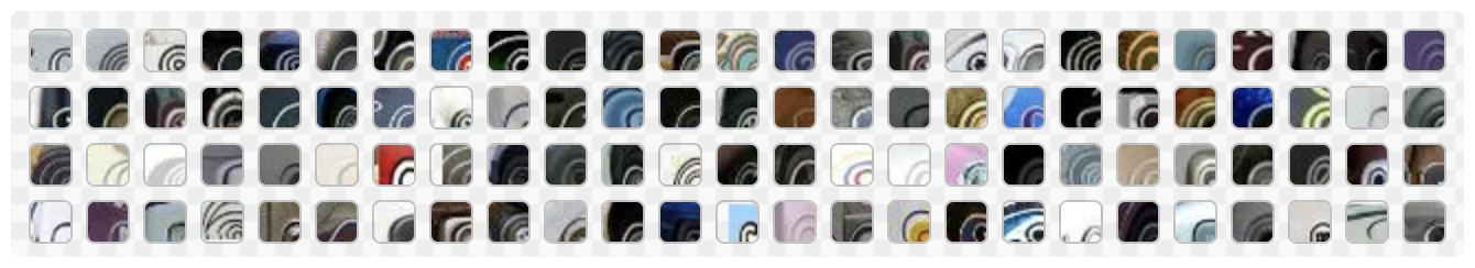
To understand different parts of this distribution qualitatively we can render a quilt of images by activation, randomly sampling images that cause 3b:379 to activate different amounts. The quilt shows a pattern. Images that cause the strongest activations have curves that are similar to the neuron’s feature visualization. Images that cause weakly positive activations are imperfect curves, either too flat, off-orientation, or with some other defect. Images that cause pre-ReLU activations near zero tend to be straight lines or images with no arcs, although some images are of curves about 45 degrees off orientation. Finally, the images that cause the strongest negative activations have curves with an orientation more than 45 degrees away from the neuron’s ideal curve.

Quilts of images reveal patterns across a wide range of activations, but they can be misleading. Since a neuron’s activation to a receptive-field sized crop of an image is just a single number, we can’t be sure which part of the image caused it. As a result, we could be fooled by spurious correlations. For instance, since many of the images that cause 3b:379 to fire most strongly are clocks, we may think the neuron detects clocks, rather than curves.

To see why an image excites a neuron, we can use feature visualization to visualize the image’s attribution to the neuron.

Visualizing Attribution

Most of the tools we use for studying neuron families, including feature visualization, can be used in context of a particular image using attribution.

There is a significant amount of work on how to do attribution in neural networks (eg. ). These methods attempt to describe which pixels or earlier neurons are responsible for causing neurons to fire. In the general case of complex non-linear functions, there is a lot of disagreement over which attribution methods are principled and whether they are reliable . But in the linear-case, attribution is generally agreed upon, with most methods collapsing to the same answer. In a linear function of $x$, $wcdot x$

Since a neuron’s pre-activation function and bias value is a linear function of neurons in the layer before it, we can use this generally agreed upon attribution method. In particular, curve detectors in 3b’s pre-activation value is a linear function of 3a. The attribution tensor describing how all neurons in the previous layer influenced a given neuron is the activations pointwise multiplied by the weights.

We normally use feature visualization to create a superstimulus that activates a single neuron, but we can also use it to activate linear combinations of neurons. By applying feature visualization to the attribution tensor, we are creating the stimulus that maximally activates the neurons in 3a that caused 3b:379 to fire. Additionally, we will use the absolute value of the attribution tensor, which shows us features that caused the neuron to fire and also features that inhibited it. This can be useful for seeing curve-related visual properties that influenced our cure neuron, even if that influence was to make it fire less.

Combining this together gives us $text{FeatureVisualization}(text{abs}(W odot h_{prev}))$

We can also use attribution to revisit the earlier quilt of dataset examples in more depth, seeing why each image caused 3b:379 to fire. You can click the figure to toggle between seeing raw images and attribution vector feature visualizations.

←

more negative activations

Random Dataset Images by

3b:379 Attribution

more positive activations

→

Reproduce in a Notebook

While the above experiment visualizes every neuron in 3a, attribution is a powerful and flexible tool that could be used to apply to studies of circuits in a variety of ways. For instance, we could visualize how an image flows through each neuron family in early vision before 3b, visualizing the image’s activation vector and attribution vector to curve neurons at each family along the way. Each activation vector would show what a family saw in the image, and each attribution vector would show us how it contributed to activating 3b:379.

In the next section we’ll look at a less sophisticated technique for extracting information from dataset images: blindfolding yourself from seeing neuron activations and classifying images by hand.

Human Comparison

Nick Cammarata, an author of this paper, manually labelled over 800 images into four groups: curve, imperfect curve, unrelated image, or opposing curve. We randomly sampled a fixed number of images from 3b:379 activations in bins of 100We did not cherry-pick from these bins. The data in this paper is from our first sampling of images.. While labeling, Nick could only see the image’s pixels, not additional information such as the neuron’s activations or attribution visualizations. He used the following rubric in labeling:

• Curves: The Image has a curve with a similar orientation to the neuron’s feature visualization. The curve goes across most of the width of the image.

• Imperfect Curve: The image has a curve that is similar to the neuron’s feature visualization, but has at least one significant defect. Perhaps it is too flat, has an angle interrupting the arc, or the orientation is slightly off.

• Unrelated: The image doesn’t have a curve.

• Opposing Curve: The image has a curve that differs from the neuron’s feature visualization by more than 45 degrees.

After hand-labeling these images, we compared our labels to 3b:379 activations across the same images. Using a stackplot we see that different labels separate cleanly into different activationsInterestingly, during labeling Nick felt it was often difficult to place samples into groups, as many images seemed to fall within the boundaries of the rubric. We were surprised when we saw that activations clearly separate into different levels of activation..

Still, there are many images that cause the neuron to activate but aren’t classified as curves or imperfect curves. When we visualize attribution to 3b:379 we see that many of the images contain subtle curves.

Nick found it hard to detect subtle curves across hundreds of curve images because he started to experience the Afterimage effect that occurs when looking at one kind of stimulus for a long time. As a result, he found it hard to tell whether subtle curves were simply perceptual illusions. By visualizing attribution, we can reveal the curves that the neuron sees in the image, showing us curves that our labeling process missed. In these cases, it seems 3b:379 is a superhuman curve detector.

How important are different points on the activation spectrum?

These charts are helpful for comparing our hand-labelled labels but they give an incomplete picture. While 3b:379 seems to be highly selective for curve stimuli when it fires strongly, this is only a tiny fraction of cases where it fires. Most of the time, it doesn’t fire at all, and when it does it’s usually very weakly.

To see this, we can look at the probability density over activation magnitudes from all ImageNet examples, split into the same per-activation-magnitude (x-axis) ratio of classes as our hand labelled dataset.

From this perspective, we can’t even see the cases where our neuron fires strongly! Probability density exponentially decays as we move right, and so these activations are rare. To some extent, this is what we should expect if these neurons really detect curves, since clear-cut curves rarely occur in images.

Perhaps more concerning is that, although curves are a small fraction of the cases where 3b:379 only weakly fire or didn’t fire, this graph seems to show that the majority of stimuli classified as curves also fall in these cases, as a result of neurons firing strongly being many orders of magnitude rarer. This seems to be at least partly due to labeling error and the rarity of curves (see discussion later). But it makes things a bit hard to reason about. This is why we haven’t provided a precision-recall curve: recall would be dominated by the cases where the neuron didn’t fire strongly and be dominated by potential labeling error as a result.

It’s not clear that probability density is really the right way to think about the behavior of a neuron. The vast majority of cases are cases where the neuron didn’t fire: are those actually important to think about? And if a neuron frequently barely fires, how important is that for understanding the role of a neuron in the network?

An alternative measure for thinking about the importance of different parts of the activation spectrum is contribution to expected value, $x*p(x)$

When we looked at probability density earlier, one might have been skeptical that 3b:379 was really a curve detector in a meaningful sense. Even if it’s highly selective when it fires strongly, how can that be what matters when it isn’t even visible on a probability density plot? Contribution to expected value shows us that even by a conservative measure, curves and imperfect curves form 55%. This seems consistent with the hypothesis that it really is a curve detector, and the other stimuli causing it to fire are labeling errors or cases where noisy images cause the neuron to misfire.

Our experiments studying the dataset so far has shown us that 3b:379 activations seem to correspond roughly to a human labelled judgement of whether images contain curves. Additionally, visualizing the attribution vector of these images tells us that the reason these images fire is because of the curves in the images, and we’re not being fooled by spurious correlations. But these experiments are not enough to defend the claim that curve neurons detect images of curves. Since images of curves appear infrequently in the dataset, using it to systematically study curve images is difficult. Our next few experiments will focus on this directly, studying how curve neurons respond to the space of reasonable curve images.

Joint Tuning Curves

Our first two experiments suggest that each curve detector responds to curves at a different orientation. Our next experiment will help verify that they really do detect rotated versions of the same feature, and characterize how sensitive each unit is to changes in orientation.

We do this by creating a joint tuning curveIn neuroscience, tuning curves — charts of neural response to a continuous stimulus parameter — came to prominence in the early days of vision research. Observation of receptive fields and orientation-specific responses in neurons gave rise to some of the earliest theories about how low-level visual features might combine to create higher-level representations. Since then they have been a mainstay technique in the field. of how all curve detectors respond if we rotate natural dataset examples that caused a particular curve detector to fire.

Each neuron has a gaussian-like bump surrounding it’s preferred orientation, and as
each one stops firing another starts fire, jointly spanning all orientations of curves.

Neuron Responses to Rotated Dataset Examples

We collect dataset examples that maximally activate neuron. We rotate them by increments of 1 degree from 0 to 360 degrees and record activations.

The activations are shifted so that the points where each neuron responds are aligned. The curves are then averaged to create a typical response curve.

While tuning curves are useful for measuring neuron activations across perturbations in natural images, we’re limited by the kinds of perturbations we can do on these images. In our next experiment we’ll get access to a larger range of perturbations by rendering artificial stimuli from scratch.

Synthetic Curves

While the dataset gives us almost every imaginable curve, they don’t come labelled with data such as orientation or radius, making it hard to answer questions that require systematically measuring responses to visual properties. How sensitive are curve detectors to curvature? What orientations do they respond to? Does it matter what colors are involved? One way to get more insight into these questions is to draw our own curves. Using synthetic stimuli like this is a common method in visual neuroscience, and we’ve found it to also be very helpful in the study of artificial neural networks. The experiments in this section are specifically inspired by similar experiments probing for curve detecting biological neurons .

Since dataset examples suggest curve detectors are most sensitive to orientation and curvature, we’ll use them as parameters in our curve renderer. We can use this to measure how changes in each property causes a given neuron, such as 3b:379, to fire. We find it helpful to present this as a heatmap, in order to get a higher resolution perspective on what causes the neuron to fire.

0σ

Standard Deviations

25σ

We find that simple drawings can be extraordinarily exciting. The curve images that cause the strongest excitations — up to 24 standard deviations above the average dataset activation! — have similar orientation and curvature to the neuron’s feature visualization.

0σ

Standard Deviations

25σ

Reproduce in a Notebook

Why do we see wispy triangles?

The triangular geometry shows that curve detectors respond to a wider range of orientations in curves with higher curvature. This is because curves with more curvature contain more orientations. Consider that a line contains no curve orientations and a circle contains every curve orientation. Since the synthetic images closer to the top are closer to lines, their activations are more narrow.

The wisps show that tiny changes in orientation or curvature can cause dramatic changes in activations, which indicate that curve detectors are fragile and non-robust. Sadly, this is a more general problem across neuron families, and we see it as early as the Gabor family in the second layer (conv2d1).

Varying curves along just two variables reveals barely-perceptible perturbations that sway activations several standard deviations. This suggests that the higher dimensional pixel-space contains more pernicious exploits. We’re excited about the research direction of carefully studying neuron-specific adversarial attacks, particularly in early vision. One benefit of studying early vision families is that it’s tractible to follow the whole circuit back to the input, and this could be made simpler by extracting the important parts of a circuit and studying it in isolation. Perhaps this simplified environment could give us clues into how to make neurons more robust or even protect whole models against adversarial attacks.

In addition to testing orientation and curvature, we can also test other variants like whether the curve shapes are filled, or if they have color. Dataset analyses hints that curve detectors are invariant to cosmetic properties like lighting, and color, and we can confirm this with synthetic stimuli.

Curves are invariant to fill..

..as well as color

0σ

Standard Deviations

25σ

Synthetic Angles

Both our synthetic curve experiments and dataset analysis show that although curves are sensitive to orientation, they have a wide tolerance for the radius of curves. At the extreme, curve neurons partially respond to edges in a narrow band of orientations, which can be seen as a curve with infinite radius. This may cause us to think curve neurons actually respond to lots of shapes with the right orientation, rather than curves specifically. While we cannot systematically render all possible shapes, we think angles are a good test case for studying this hypothesis.

In the following experiment we vary synthetic angles similarly to our synthetic curves, with radius on the y axis and orientation across the x axis.

0σ

Standard Deviations

25σ

The activations form two distinct lines, with the strongest activations where they touch. Each line is where one of the two lines in the angle aligns with the tangent of the curve. The two lines touch where the angle most similar to a curve with an orientation that matches the neuron’s feature visualization. The weaker activations on the right side of the activations have the same cause, but with the inhibitory half of the angle stimulus facing outwards instead of inwards.

The first stimuli we looked at were synthetic curves and the second stimuli was synthetic angles. In the next examples we show a series of stimuli that transition from angles to curves. Each column’s strongest activation is stronger than the column before it since rounder stimuli are closer to curves, causing curve neurons to fire more strongly. Additionally, as each stimulus becomes rounder, their “triangles of activation” become increasingly filled as the two lines from the original angle stimuli transition into a smooth arc.

0σ

Standard Deviations

25σ

Reproduce in a Notebook

This interface is useful for seeing how different curve neurons respond to changes in multiple stimuli properties, but it’s bulky. In the next section we’ll be exploring curve families across different layers, and it will be helpful to have a more compact way to view activations of a curve neuron family. For this, we’ll introduce a radial tuning curve.

Radial Tuning Curve

Hover to isolate a neuron

The Curve Families of InceptionV1

So far we’ve been looking at a set of curve neurons in 3b. But InceptionV1 actually contains curve neurons in four contiguous layers, with 3b being the third of these layers.

conv2d2

“conv2d2”, which we sometimes shorten to “2″, is the third convolutional layer in InceptionV1. It contains two types of curve detectors: concentric curves and combed edges.

Concentric curves are small curve detectors that have a preference for multiple curves at the same orientation with increasing radii. We believe this feature has a role in the development of curve detectors in 3a and 3b that are tolerant of a wide range of radii.

Combed edges detect several lines protruding perpendicularly from a larger line. These protruding lines also detect curves, making them a type of curve detector. These neurons are used to construct later curve detectors and play a part in the combing effect.

Looking at conv2d2 activations we see that curves respond to one contiguous range like the ones in 3b, but also weakly activate to a range on the opposite side, 180 degrees away. We call this secondary range echoes.

3a

By 3a non-concentric curve detectors have formed. In many ways they resemble the curve detectors in 3b, and in the next article we’ll see how they’re used to build 3b curves. One difference is that the 3a curves have echoes.

3b

These are the curve detectors we’ve been focusing on in this article. They have clean activations with no echoes.

You may notice that there are two large angular gaps at the top of the radial tuning curve for 3b, and smaller ones at the bottom. Why is that? One factor is that the model also has what we call double curve detectors which respond to curves in two different orientations and help fill in the gaps.

4a

In 4a the network constructs many complex shapes such as spirals and boundary detectors, and it is also the first layer to construct 3d geometry. It has several curve detectors, but we believe they are better thought of as corresponding to specific worldly objects rather than abstract shapes. Many of these curves are found in 4a’s 5×5 branch, which seems to specialize in 3d geometry.

For instance, 4a:406 appears to be a upwards facing curve detector with confusing secondary behavior at two other angles. But dataset examples reveal its secret: it’s detecting the tops of cups and pans viewed from an angle. In this sense, it is better viewed as a tilted 3d circle detector.

We think 4a:406 is a good example of how neural network interpretability can be subjective. We usually think of abstract concepts like curves and worldly objects like coffee cups as belonging as different kinds of things — and for most of the network they are separate. But there’s a transition period where we have to make a judgement call, and 4a is that transition.

Repurposing Curve Detectors

We started studying curve neurons to better understand neural networks, not because we were intrinsically interested in curves. But during our investigation we became aware that curve detection is important for fields like aerial imaging, self-driving cars, and medical research, and there’s a breadth of literature from classical computer vision on curve detection in each domain. We’ve prototyped a technique that leverages the curve neuron family to do a couple different curve related computer vision tasks.

One task is curve extraction  , the task of highlighting the pixels of the image that are part of curves. Visualizing attribution to curve neurons, as we’ve been doing in this article, can be seen as a form of curve extraction. Here we compare it to the commonly used Canny edge detection algorithm on an x-ray of blood vessels known as an angiogram, taken from  , Figure 2.1.

The attribution visualization clearly separates and illuminates the lines and curves, and displays less visual artifacts. However, it displays a strong combing effect — unwanted perpendicular lines emanating from the edge being traced. We’re unsure how harmful these lines are in practice for this application, but we think it’s possible to remove them by editing the circuits of curve neurons.

We don’t mean to suggest we’ve created a competitive curve tracing algorithm. We haven’t done a detailed comparison to state of the art curve detection algorithms, and believe it’s likely that classical algorithms tuned for precisely this goal outperform our approach. Instead, our goal here is to explore how leveraging internal neural network representations opens a vast space of visual operations, of which curve extraction is just one point.

Spline Parameterization

We can access more parts of this space by changing what we optimize. So far we’ve been optimizing pixels, but we can also create a differentiable parameterization that renders curves, similar to explorations by and . By backpropagating from the attribution through the input into spline knots, we can now trace curves — obtaining the equations of the best fitting spline equations that describe the curves in the image.

We created an early prototype of this approach. Since curve neurons work in a variety of settingsAs we explored in the article, curve neurons are robust to cosmetic properties like brightness and texture., our spline parameterization does too.

Occlusion

Subtle Curve

Complex Shapes

Reproduce in a Notebook

Algorithmic Composition

One seemingly unrelated visual operation is image segmentation. This can be done in an unsupervised way using non-negative matrix factorization (NMF) . We can visualize attribution to each of these factors with our spline parameterization to trace the curves of different objects in the image.

Instead of factoring the activations of a single image, we can jointly factorize lots of butterflies to find the neurons in the network that respond to butterflies in general. One big difference between factoring activations and normal image segmentation is that we get groups of neurons rather than pixels. These neuron groups can be applied to find butterflies in images in general, and by composing this with differentiable spline parameterization we get a single optimization we can apply to any image that automatically finds butterflies and gives us equations to splines that fit them.

Reproduce in a Notebook

In this above example we manipulated butterflies and curves without having to worry about the details of either. We delegated the intricacies of recognizing butterflies of many species and orientations to the neurons, letting us work with the abstract concept of butterflies.

We think this is one exciting way to fuse classical computer vision with deep learning. There is plenty of low hanging fruit in extending the technique shown above, as our spline parameterization is just an early prototype and our optimizations are using a neural network that’s half a decade old. However, we’re more excited by investigations of how users can explore the space between tasks than improvements in any particular task. Once a task is set in stone, training a neural network for exactly that job will likely give the best results. But real world tasks are rarely specified with precision, and the harder challenge is to explore the space of tasks to find which to commit to.

For instance, a more developed version of our algorithm that automatically finds the splines of butterflies in an image could be used as a basis for turning video footage of butterflies into an animationUsing a shared parameterization to maintain consistency between frames.. But an animator may wish to add texture neurons and change to a soft brush parameterization to add a rotoscoping style to their animation. Since they have full access to every neuron in the render, they could manipulate attribution to fur neuron families and specific dog breeds, changing how fur is rendered on specific species of dogs across the entire movie. Since none of these algorithms require retraining a neural network or any training data, in-principle an animator could explore this space of algorithms in real time, which is important because tight feedback loops can be crucial in unlocking creative potential.

The Combing Phenomenon

One curious aspect of curve detectors is that they seem to be excited by small lines perpendicular to the curve, both inwards and outwards. You can see this most easily by inspecting feature visualizations. We call this phenomenon “combing.”

Combing seems to occur across curve detectors from many models, including models trained on Places365 instead of ImageNet. In fact, there’s some weak evidence it occurs in biological neural networks as well: a team that ran a process similar to feature visualization on a biological neuron in a Macaque monkey’s V4 region of the visual cortex found a circular shape with outwardly protruding lines to be one of the highest activating stimuli.

AlexNet

InceptionV1

InceptionV3

Monkey V4

A number of potential explanations for combing have been proposed, with no clear forerunner.

One hypothesis is that many important curves in the modern world have perpendicular lines, such as the spokes of a wheel or the markings on the rim of a clock.

A related hypothesis is that combing might allow curve detectors to be used for fur detection in some contexts. Another hypothesis is that a curve has higher “contrast” with perpendicular lines running towards. Recall that in the dataset examples, the strongest negative pre-ReLU activations were curves at opposite orientations. If a curve detector wants to see a strong change in orientation between the curve and the space around it, it may consider perpendicular lines to be more contrast than a solid color.

Finally, we think it’s possible that combing is really just a convenient way to implement curve detectors — a side effect of a shortcut in circuit construction rather than an intrinsically useful feature. In conv2d1, edge detectors are inhibited by perpendicular lines in conv2d0. One of the things a line or curve detector needs to do is check that the image is not just a single repeating texture, but that it has a strong line surrounded by contrast. It seems to do this by weakly inhibiting parallel lines alongside the tangent. Being excited by a perpendicular line may be an easy way to implement a “inhibit an excitatory neuron” pattern which allows for capped inhibition, without creating dedicated neurons at the previous layer.

Combing is not unique to curves. We also observe it in lines, and basically any shape feature like curves that is derivative of lines. A lot more work could be done exploring the combing phenomenon. Why does combing form? Does it persist in adversarially robust models? Is it an example of what Ilyas et al call a “non-robust feature”?

Conclusion

Compared to fields like neuroscience, artificial neural networks make careful investigation easy. We can read and write to every weight in the neural network, use gradients to optimize stimuli, and analyze billions of realistic activations across a dataset. Composing these tools lets us run a wide range of experiments that show us different perspectives on a neuron. If every perspective shows the same story, it’s unlikely we’re missing something big.

Given this, it may seem odd to invest so much energy into just a handful of neurons. We agree. We first estimated it would take a week to understand the curve family. Instead, we spent months exploring the fractal of beauty and structure we found.

Many paths led to new techniques for studying neurons in general, like synthetic stimuli or using circuit editing to ablate neurons behavior. Others are only relevant for some families, such as the equivariance motif or our hand-trained “artificial artificial neural network” that reimplements curve detectors. A couple were curve-specific, like exploring curve detectors as a type of curve analysis algorithms.

If our broader goal is fully reverse-engineer neural networks it may seem concerning that studying just one family took so much effort. However, from our experience studying neuron families at a variety of depths, we’ve found that it’s easy to understand the basics of a neuron family. OpenAI Microscope shows you feature visualizations, dataset examples, and soon weights in just a few seconds. Since feature visualization shows strong evidence of causal behavior and dataset examples show what neurons respond to in practice, these are collectively strong evidence of what a neuron does. In fact, we understood the basics of curves at our first glance at them.

While it’s usually possible to understand the main function of a neuron family at a glance, researchers engaging in closer inquiry of neuron families will be rewarded with deeper beauty.
When we started, we were nervous that 10 neurons was too narrow a topic for a paper, but now we realize a complete investigation would take a book.

This article is part of the Circuits thread, an experimental format collecting invited short articles and critical commentary delving into the inner workings of neural networks.

An Overview of Early Vision in InceptionV1Naturally Occurring Equivariance in Neural Networks