Many real-world problems require integrating multiple sources of information.
Sometimes these problems involve multiple, distinct modalities of
information — vision, language, audio, etc. — as is required
to understand a scene in a movie or answer a question about an image.
Other times, these problems involve multiple sources of the same
kind of input, i.e. when summarizing several documents or drawing one
image in the style of another.

When approaching such problems, it often makes sense to process one source
of information in the context of another; for instance, in the
right example above, one can extract meaning from the image in the context
of the question. In machine learning, we often refer to this context-based
processing as conditioning: the computation carried out by a model
is conditioned or modulated by information extracted from an
auxiliary input.

Finding an effective way to condition on or fuse sources of information
is an open research problem, and

in this article, we concentrate on a specific family of approaches we call
feature-wise transformations.

We will examine the use of feature-wise transformations in many neural network
architectures to solve a surprisingly large and diverse set of problems;

their success, we will argue, is due to being flexible enough to learn an
effective representation of the conditioning input in varied settings.
In the language of multi-task learning, where the conditioning signal is
taken to be a task description, feature-wise transformations
learn a task representation which allows them to capture and leverage the
relationship between multiple sources of information, even in remarkably
different problem settings.

Feature-wise transformations

To motivate feature-wise transformations, we start with a basic example,
where the two inputs are images and category labels, respectively. For the
purpose of this example, we are interested in building a generative model of
images of various classes (puppy, boat, airplane, etc.). The model takes as
input a class and a source of random noise (e.g., a vector sampled from a
normal distribution) and outputs an image sample for the requested class.

Our first instinct might be to build a separate model for each
class. For a small number of classes this approach is not too bad a solution,
but for thousands of classes, we quickly run into scaling issues, as the number
of parameters to store and train grows with the number of classes.
We are also missing out on the opportunity to leverage commonalities between
classes; for instance, different types of dogs (puppy, terrier, dalmatian,
etc.) share visual traits and are likely to share computation when
mapping from the abstract noise vector to the output image.

Now let’s imagine that, in addition to the various classes, we also need to
model attributes like size or color. In this case, we can’t
reasonably expect to train a separate network for each possible
conditioning combination! Let’s examine a few simple options.

A quick fix would be to concatenate a representation of the conditioning
information to the noise vector and treat the result as the model’s input.
This solution is quite parameter-efficient, as we only need to increase
the size of the first layer’s weight matrix. However, this approach makes the implicit
assumption that the input is where the model needs to use the conditioning information.
Maybe this assumption is correct, or maybe it’s not; perhaps the
model does not need to incorporate the conditioning information until late
into the generation process (e.g., right before generating the final pixel
output when conditioning on texture). In this case, we would be forcing the model to
carry this information around unaltered for many layers.

Because this operation is cheap, we might as well avoid making any such
assumptions and concatenate the conditioning representation to the input of
all layers in the network. Let’s call this approach
concatenation-based conditioning.

Another efficient way to integrate conditioning information into the network
is via conditional biasing, namely, by adding a bias to
the hidden layers based on the conditioning representation.

Interestingly, conditional biasing can be thought of as another way to
implement concatenation-based conditioning. Consider a fully-connected
linear layer applied to the concatenation of an input
$mathbf{x}$ and a conditioning representation
$mathbf{z}$:

The same argument applies to convolutional networks, provided we ignore
the border effects due to zero-padding.

Yet another efficient way to integrate class information into the network is
via conditional scaling, i.e., scaling hidden layers
based on the conditioning representation.

A special instance of conditional scaling is feature-wise sigmoidal gating:
we scale each feature by a value between $0$ and
$1$ (enforced by applying the logistic function), as a
function of the conditioning representation. Intuitively, this gating allows
the conditioning information to select which features are passed forward
and which are zeroed out.

Given that both additive and multiplicative interactions seem natural and
intuitive, which approach should we pick? One argument in favor of
multiplicative interactions is that they are useful in learning
relationships between inputs, as these interactions naturally identify
“matches”: multiplying elements that agree in sign yields larger values than
multiplying elements that disagree. This property is why dot products are
often used to determine how similar two vectors are.

Multiplicative interactions alone have had a history of success in various
domains — see Bibliographic Notes.

One argument in favor of additive interactions is that they are
more natural for applications that are less strongly dependent on the
joint values of two inputs, like feature aggregation or feature detection
(i.e., checking if a feature is present in either of two inputs).

In the spirit of making as few assumptions about the problem as possible,
we may as well combine both into a
conditional affine transformation.

An affine transformation is a transformation of the form
$y = m * x + b$.

All methods outlined above share the common trait that they act at the
feature level; in other words, they leverage feature-wise
interactions between the conditioning representation and the conditioned
network. It is certainly possible to use more complex interactions,
but feature-wise interactions often strike a happy compromise between
effectiveness and efficiency: the number of scaling and/or shifting
coefficients to predict scales linearly with the number of features in the
network. Also, in practice, feature-wise transformations (often compounded
across multiple layers) frequently have enough capacity to model complex
phenomenon in various settings.

Lastly, these transformations only enforce a limited inductive bias and
remain domain-agnostic. This quality can be a downside, as some problems may
be easier to solve with a stronger inductive bias. However, it is this
characteristic which also enables these transformations to be so widely
effective across problem domains, as we will later review.

Nomenclature

To continue the discussion on feature-wise transformations we need to
abstract away the distinction between multiplicative and additive
interactions. Without losing generality, let’s focus on feature-wise affine
transformations, and let’s adopt the nomenclature of Perez et al.
, which formalizes conditional affine
transformations under the acronym FiLM, for Feature-wise Linear
Modulation.

Strictly speaking, linear is a misnomer, as we allow biasing, but
we hope the more rigorous-minded reader will forgive us for the sake of a
better-sounding acronym.

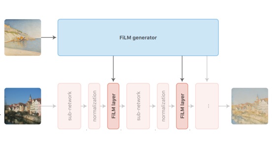
We say that a neural network is modulated using FiLM, or FiLM-ed,
after inserting FiLM layers into its architecture. These layers are
parametrized by some form of conditioning information, and the mapping from
conditioning information to FiLM parameters (i.e., the shifting and scaling
coefficients) is called the FiLM generator.
In other words, the FiLM generator predicts the parameters of the FiLM
layers based on some auxiliary input.
Note that the FiLM parameters are parameters in one network but predictions
from another network, so they aren’t learnable parameters with fixed
weights as in the fully traditional sense.
For simplicity, you can assume that the FiLM generator outputs the
concatenation of all FiLM parameters for the network architecture.

As the name implies, a FiLM layer applies a feature-wise affine
transformation to its input. By feature-wise, we mean that scaling
and shifting are applied element-wise, or in the case of convolutional
networks, feature map -wise.

To expand a little more on the convolutional case, feature maps can be
thought of as the same feature detector being evaluated at different
spatial locations, in which case it makes sense to apply the same affine
transformation to all spatial locations.

In other words, assuming $mathbf{x}$ is a FiLM layer’s
input, $mathbf{z}$ is a conditioning input, and
$gamma$ and $beta$ are
$mathbf{z}$-dependent scaling and shifting vectors,

$textrm{FiLM}(mathbf{x}) = gamma(mathbf{z}) odot mathbf{x} + beta(mathbf{z}).$

You can interact with the following fully-connected and convolutional FiLM
layers to get an intuition of the sort of modulation they allow:

In addition to being a good abstraction of conditional feature-wise
transformations, the FiLM nomenclature lends itself well to the notion of a
task representation. From the perspective of multi-task learning,
we can view the conditioning signal as the task description. More
specifically, we can view the concatenation of all FiLM scaling and shifting
coefficients as both an instruction on how to modulate the
conditioned network and a representation of the task at hand. We
will explore and illustrate this idea later on.

Feature-wise transformations in the literature

Feature-wise transformations find their way into methods applied to many
problem settings, but because of their simplicity, their effectiveness is
seldom highlighted in lieu of other novel research contributions. Below are
a few notable examples of feature-wise transformations in the literature,
grouped by application domain. The diversity of these applications
underscores the flexible, general-purpose ability of feature-wise
interactions to learn effective task representations.

expand all

Visual question-answering+

Perez et al. use
FiLM layers to build a visual reasoning model
trained on the CLEVR dataset to
answer multi-step, compositional questions about synthetic images.

The model’s linguistic pipeline is a FiLM generator which
extracts a question representation that is linearly mapped to
FiLM parameter values. Using these values, FiLM layers inserted within each
residual block condition the visual pipeline. The model is trained
end-to-end on image-question-answer triples. Strub et al.
later on improved on the model by
using an attention mechanism to alternate between attending to the language
input and generating FiLM parameters layer by layer. This approach was
better able to scale to settings with longer input sequences such as
dialogue and was evaluated on the GuessWhat?!
and ReferIt datasets.

de Vries et al. leverage FiLM
to condition a pre-trained network. Their model’s linguistic pipeline
modulates the visual pipeline via conditional batch normalization,
which can be viewed as a special case of FiLM. The model learns to answer natural language questions about
real-world images on the GuessWhat?!
and VQAv1 datasets.

The visual pipeline consists of a pre-trained residual network that is
fixed throughout training. The linguistic pipeline manipulates the visual
pipeline by perturbing the residual network’s batch normalization
parameters, which re-scale and re-shift feature maps after activations
have been normalized to have zero mean and unit variance. As hinted
earlier, conditional batch normalization can be viewed as an instance of
FiLM where the post-normalization feature-wise affine transformation is
replaced with a FiLM layer.

Style transfer+

Dumoulin et al. use
feature-wise affine transformations — in the form of conditional
instance normalization layers — to condition a style transfer
network on a chosen style image. Like conditional batch normalization
discussed in the previous subsection,
conditional instance normalization can be seen as an instance of FiLM
where a FiLM layer replaces the post-normalization feature-wise affine
transformation. For style transfer, the network models each style as a separate set of
instance normalization parameters, and it applies normalization with these
style-specific parameters.

Dumoulin et al. use a simple
embedding lookup to produce instance normalization parameters, while
Ghiasi et al. further
introduce a style prediction network, trained jointly with the
style transfer network to predict the conditioning parameters directly from
a given style image. In this article we opt to use the FiLM nomenclature
because it is decoupled from normalization operations, but the FiLM
layers used by Perez et al. were
themselves heavily inspired by the conditional normalization layers used
by Dumoulin et al. .

Yang et al. use a related
architecture for video object segmentation — the task of segmenting a
particular object throughout a video given that object’s segmentation in the
first frame. Their model conditions an image segmentation network over a
video frame on the provided first frame segmentation using feature-wise
scaling factors, as well as on the previous frame using position-wise
biases.

So far, the models we covered have two sub-networks: a primary
network in which feature-wise transformations are applied and a secondary
network which outputs parameters for these transformations. However, this
distinction between FiLM-ed network and FiLM generator
is not strictly necessary. As an example, Huang and Belongie
propose an alternative
style transfer network that uses adaptive instance normalization layers,
which compute normalization parameters using a simple heuristic.

Adaptive instance normalization can be interpreted as inserting a FiLM
layer midway through the model. However, rather than relying
on a secondary network to predict the FiLM parameters from the style
image, the main network itself is used to extract the style features
used to compute FiLM parameters. Therefore, the model can be seen as
both the FiLM-ed network and the FiLM generator.

Image recognition+

As discussed in previous subsections, there is nothing preventing us from considering a
neural network’s activations themselves as conditioning
information. This idea gives rise to
self-conditioned models.

Highway Networks are a prime
example of applying this self-conditioning principle. They take inspiration
from the LSTMs’ heavy use of
feature-wise sigmoidal gating in their input, forget, and output gates to
regulate information flow:

The ImageNet 2017 winning model also
employs feature-wise sigmoidal gating in a self-conditioning manner, as a
way to “recalibrate” a layer’s activations conditioned on themselves.

Natural language processing+

For statistical language modeling (i.e., predicting the next word
in a sentence), the LSTM
constitutes a popular class of recurrent network architectures. The LSTM
relies heavily on feature-wise sigmoidal gating to control the
information flow in and out of the memory or context cell
$mathbf{c}$, based on the hidden states
$mathbf{h}$ and inputs $mathbf{x}$ at
every timestep $mathbf{t}$.

Also in the domain of language modeling, Dauphin et al. use sigmoidal
gating in their proposed gated linear unit, which uses half of the
input features to apply feature-wise sigmoidal gating to the other half.
Gehring et al. adopt this
architectural feature, introducing a fast, parallelizable model for machine
translation in the form of a fully convolutional network.

The Gated-Attention Reader
uses feature-wise scaling, extracting information
from text by conditioning a document-reading network on a query. Its
architecture consists of multiple Gated-Attention modules, which involve
element-wise multiplications between document representation tokens and
token-specific query representations extracted via soft attention on the
query representation tokens.

Reinforcement learning+

The Gated-Attention architecture
uses feature-wise sigmoidal gating to fuse linguistic and visual
information in an agent trained to follow simple “go-to” language
instructions in the VizDoom 3D
environment.

Bahdanau et al. use FiLM
layers to condition Neural Module Network
and LSTM -based policies to follow
basic, compositional language instructions (arranging objects and going
to particular locations) in a 2D grid world. They train this policy
in an adversarial manner using rewards from another FiLM-based network,
trained to discriminate between ground-truth examples of achieved
instruction states and failed policy trajectories states.

Outside instruction-following, Kirkpatrick et al.
also use
game-specific scaling and biasing to condition a shared policy network
trained to play 10 different Atari games.

Generative modeling+

The conditional variant of DCGAN ,
a well-recognized network architecture for generative adversarial networks
, uses concatenation-based
conditioning. The class label is broadcasted as a feature map and then
concatenated to the input of convolutional and transposed convolutional
layers in the discriminator and generator networks.

For convolutional layers, concatenation-based conditioning requires the
network to learn redundant convolutional parameters to interpret each
constant, conditioning feature map; as a result, directly applying a
conditional bias is more parameter efficient, but the two approaches are
still mathematically equivalent.

PixelCNN
and WaveNet  — two recent
advances in autoregressive, generative modeling of images and audio,
respectively — use conditional biasing. The simplest form of
conditioning in PixelCNN adds feature-wise biases to all convolutional layer
outputs. In FiLM parlance, this operation is equivalent to inserting FiLM
layers after each convolutional layer and setting the scaling coefficients
to a constant value of 1.

The authors also describe a location-dependent biasing scheme which
cannot be expressed in terms of FiLM layers due to the absence of the
feature-wise property.

WaveNet describes two ways in which conditional biasing allows external
information to modulate the audio or speech generation process based on
conditioning input:

1. Global conditioning applies the same conditional bias
   to the whole generated sequence and is used e.g. to condition on speaker
   identity.
2. Local conditioning applies a conditional bias which
   varies across time steps of the generated sequence and is used e.g. to
   let linguistic features in a text-to-speech model influence which sounds
   are produced.

As in PixelCNN, conditioning in WaveNet can be viewed as inserting FiLM
layers after each convolutional layer. The main difference lies in how
the FiLM-generating network is defined: global conditioning
expresses the FiLM-generating network as an embedding lookup which is
broadcasted to the whole time series, whereas local conditioning expresses
it as a mapping from an input sequence of conditioning information to an
output sequence of FiLM parameters.

Speech recognition+

Kim et al. modulate a deep
bidirectional LSTM using a form
of conditional normalization. As discussed in the
Visual question-answering and Style transfer subsections,
conditional normalization can be seen as an instance of FiLM where
the post-normalization feature-wise affine transformation is replaced
with a FiLM layer.

The key difference here is that the conditioning signal does not come from
an external source but rather from utterance
summarization feature vectors extracted in each layer to adapt the model.

Domain adaptation and few-shot learning+

For domain adaptation, Li et al.
find it effective to update the per-channel batch normalization
statistics (mean and variance) of a network trained on one domain with that
network’s statistics in a new, target domain. As discussed in the
Style transfer subsection, this operation is akin to using the network as
both the FiLM generator and the FiLM-ed network. Notably, this approach,
along with Adaptive Instance Normalization, has the particular advantage of
not requiring any extra trainable parameters.

For few-shot learning, Oreshkin et al.
explore the use of FiLM layers to
provide more robustness to variations in the input distribution across
few-shot learning episodes. The training set for a given episode is used to
produce FiLM parameters which modulate the feature extractor used in a
Prototypical Networks
meta-training procedure.

Aside from methods which make direct use of feature-wise transformations,
the FiLM framework connects more broadly with the following methods and
concepts.

expand all

Zero-shot learning+

The idea of learning a task representation shares a strong connection with
zero-shot learning approaches. In zero-shot learning, semantic task
embeddings may be learned from external information and then leveraged to
make predictions about classes without training examples. For instance, to
generalize to unseen object categories for image classification, one may
construct semantic task embeddings from text-only descriptions and exploit
objects’ text-based relationships to make predictions for unseen image
categories. Frome et al. , Socher et
al. , and Norouzi et al.
are a few notable exemplars
of this idea.

HyperNetworks+

The notion of a secondary network predicting the parameters of a primary
network is also well exemplified by HyperNetworks , which predict weights for entire layers
(e.g., a recurrent neural network layer). From this perspective, the FiLM
generator is a specialized HyperNetwork that predicts the FiLM parameters of
the FiLM-ed network. The main distinction between the two resides in the
number and specificity of predicted parameters: FiLM requires predicting far
fewer parameters than Hypernetworks, but also has less modulation potential.
The ideal trade-off between a conditioning mechanism’s capacity,
regularization, and computational complexity is still an ongoing area of
investigation, and many proposed approaches lie on the spectrum between FiLM
and HyperNetworks (see Bibliographic Notes).

Attention+

Some parallels can be drawn between attention and FiLM, but the two operate
in different ways which are important to disambiguate.

This difference stems from distinct intuitions underlying attention and
FiLM: the former assumes that specific spatial locations or time steps
contain the most useful information, whereas the latter assumes that
specific features or feature maps contain the most useful information.

Bilinear transformations+

With a little bit of stretching, FiLM can be seen as a special case of a
bilinear transformation
with low-rank weight
matrices. A bilinear transformation defines the relationship between two
inputs $mathbf{x}$ and $mathbf{z}$ and the
$k^{th}$

$y_k = mathbf{x}^T W_k mathbf{z}.$

Note that for each output feature $y_k$

If we view $mathbf{z}$ as the concatenation of the scaling
and shifting vectors $gamma$ and $beta$ and
if we augment the input $mathbf{x}$ with a 1-valued feature,

As is commonly done to turn a linear transformation into an affine
transformation.

we can represent FiLM using a bilinear transformation by zeroing out the
appropriate weight matrix entries:

For some applications of bilinear transformations,
see the Bibliographic Notes.

Properties of the learned task representation

As hinted earlier, in adopting the FiLM perspective we implicitly introduce
a notion of task representation: each task — be it a question
about an image or a painting style to imitate — elicits a different
set of FiLM parameters via the FiLM generator which can be understood as its
representation in terms of how to modulate the FiLM-ed network. To help
better understand the properties of this representation, let’s focus on two
FiLM-ed models used in fairly different problem settings:

• The visual reasoning model of Perez et al.
  , which uses FiLM
  to modulate a visual processing pipeline based off an input question.

  
  

• The artistic style transfer model of Ghiasi et al.
  , which uses FiLM to modulate a
  feed-forward style transfer network based off an input style image.

  
  

As a starting point, can we discern any pattern in the FiLM parameters as a
function of the task description? One way to visualize the FiLM parameter
space is to plot $gamma$ against $beta$,
with each point corresponding to a specific task description and a specific
feature map. If we color-code each point according to the feature map it
belongs to we observe the following:

The plots above allow us to make several interesting observations. First,
FiLM parameters cluster by feature map in parameter space, and the cluster
locations are not uniform across feature maps. The orientation of these
clusters is also not uniform across feature maps: the main axis of variation
can be $gamma$-aligned, $beta$-aligned, or
diagonal at varying angles. These findings suggest that the affine
transformation in FiLM layers is not modulated in a single, consistent way,
i.e., using $gamma$ only, $beta$ only, or
$gamma$ and $beta$ together in some specific
way. Maybe this is due to the affine transformation being overspecified, or
maybe this shows that FiLM layers can be used to perform modulation
operations in several distinct ways.

Nevertheless, the fact that these parameter clusters are often somewhat
“dense” may help explain why the style transfer model of Ghiasi et al.
is able to perform style
interpolations: any convex combination of FiLM parameters is likely to
correspond to a meaningful parametrization of the FiLM-ed network.

To some extent, the notion of interpolating between tasks using FiLM
parameters can be applied even in the visual question-answering setting.
Using the model trained in Perez et al. ,
we interpolated between the model’s FiLM parameters for two pairs of CLEVR
questions. Here we visualize the input locations responsible for
the globally max-pooled features fed to the visual pipeline’s output classifier:

The network seems to be softly switching where in the image it is looking,
based on the task description. It is quite interesting that these semantically
meaningful interpolation behaviors emerge, as the network has not been
trained to act this way.

Despite these similarities across problem settings, we also observe
qualitative differences in the way in which FiLM parameters cluster as a
function of the task description. Unlike the style transfer model, the
visual reasoning model sometimes exhibits several FiLM parameter
sub-clusters for a given feature map.

At the very least, this may indicate that FiLM learns to operate in ways
that are problem-specific, and that we should not expect to find a unified
and problem-independent explanation for FiLM’s success in modulating FiLM-ed
networks. Perhaps the compositional or discrete nature of visual reasoning
requires the model to implement several well-defined modes of operation
which are less necessary for style transfer.

Focusing on individual feature maps which exhibit sub-clusters, we can try
to infer how questions regroup by color-coding the scatter plots by question
type.

Sometimes a clear pattern emerges, as in the right plot, where color-related
questions concentrate in the top-right cluster — we observe that
questions either are of type Query color or Equal color,
or contain concepts related to color. Sometimes it is harder to draw a
conclusion, as in the left plot, where question types are scattered across
the three clusters.

In cases where question types alone cannot explain the clustering of the
FiLM parameters, we can turn to the conditioning content itself to gain
an understanding of the mechanism at play. Let’s take a look at two more
plots: one for feature map 26 as in the previous figure, and another
for a different feature map, also exhibiting several subclusters. This time
we regroup points by the words which appear in their associated question.

In the left plot, the left subcluster corresponds to questions involving
objects positioned in front of other objects, while the right
subcluster corresponds to questions involving objects positioned
behind other objects. In the right plot we see some evidence of
separation based on object material: the left subcluster corresponds to
questions involving matte and rubber objects, while the
right subcluster contains questions about shiny or
metallic objects.

The presence of sub-clusters in the visual reasoning model also suggests
that question interpolations may not always work reliably, but these
sub-clusters don’t preclude one from performing arithmetic on the question
representations, as Perez et al.
report.

Perez et al. report that this sort of
task analogy is not always successful in correcting the model’s answer, but
it does point to an interesting fact about FiLM-ed networks: sometimes the
model makes a mistake not because it is incapable of computing the correct
output, but because it fails to produce the correct FiLM parameters for a
given task description. The reverse can also be true: if the set of tasks
the model was trained on is insufficiently rich, the computational
primitives learned by the FiLM-ed network may be insufficient to ensure good
generalization. For instance, a style transfer model may lack the ability to
produce zebra-like patterns if there are no stripes in the styles it was
trained on. This could explain why Ghiasi et al.
report that their style transfer
model’s ability to produce pastiches for new styles degrades if it has been
trained on an insufficiently large number of styles. Note however that in
that case the FiLM generator’s failure to generalize could also play a role,
and further analysis would be needed to draw a definitive conclusion.

This points to a separation between the various computational
primitives learned by the FiLM-ed network and the “numerical recipes”
learned by the FiLM generator: the model’s ability to generalize depends
both on its ability to parse new forms of task descriptions and on it having
learned the required computational primitives to solve those tasks. We note
that this multi-faceted notion of generalization is inherited directly from
the multi-task point of view adopted by the FiLM framework.

Let’s now turn our attention back to the overal structural properties of FiLM
parameters observed thus far. The existence of this structure has already
been explored, albeit more indirectly, by Ghiasi et al.
as well as Perez et al.
, who applied t-SNE
on the FiLM parameter values.

The projection on the left is inspired by a similar projection done by Perez
et al. for their visual reasoning
model trained on CLEVR and shows how questions group by question type.
The projection on the right is inspired by a similar projection done by
Ghiasi et al. for their style
transfer network. The projection does not cluster artists as neatly as the
projection on the left, but this is to be expected, given that an artist’s
style may vary widely over time. However, we can still detect interesting
patterns in the projection: note for instance the isolated cluster (circled
in the figure) in which paintings by Ivan Shishkin and Rembrandt are
aggregated. While these two painters exhibit fairly different styles, the
cluster is a grouping of their sketches.

To summarize, the way neural networks learn to use FiLM layers seems to
vary from problem to problem, input to input, and even from feature to
feature; there does not seem to be a single mechanism by which the
network uses FiLM to condition computation. This flexibility may
explain why FiLM-related methods have been successful across such a
wide variety of domains.

Discussion

Looking forward, there are still many unanswered questions.
Do these experimental observations on FiLM-based architectures generalize to
other related conditioning mechanisms, such as conditional biasing, sigmoidal
gating, HyperNetworks, and bilinear transformations? When do feature-wise
transformations outperform methods with stronger inductive biases and vice
versa? Recent work combines feature-wise transformations with stronger
inductive bias methods
,
which could be an optimal middle ground. Also, to what extent are FiLM’s
task representation properties
inherent to FiLM, and to what extent do they emerge from other features
of neural networks (i.e. non-linearities, FiLM generator
depth, etc.)? If you are interested in exploring these or other
questions about FiLM, we recommend looking into the code bases for
FiLM models for visual reasoning
and style transfer
which we used as a
starting point for our experiments here.

Finally, the fact that changes on the feature level alone are able to
compound into large and meaningful modulations of the FiLM-ed network is
still very surprising to us, and hopefully future work will uncover deeper
explanations. For now, though, it is a question that
evokes the even grander mystery of how neural networks in general compound
simple operations like matrix multiplications and element-wise
non-linearities into semantically meaningful transformations.