Why Momentum Really Works

Industry news

2023.09.29.

Why Momentum Really Works

Step-size α = 0.02

Momentum β = 0.99

We often think of Momentum as a means of dampening oscillations and speeding up the iterations, leading to faster convergence. But it has other interesting behavior. It allows a larger range of step-sizes to be used, and creates its own oscillations. What is going on?

Here’s a popular story about momentum[1, 2, 3]: gradient descent is a man walking down a hill. He follows the steepest path downwards; his progress is slow, but steady. Momentum is a heavy ball rolling down the same hill. The added inertia acts both as a smoother and an accelerator, dampening oscillations and causing us to barrel through narrow valleys, small humps and local minima.

This standard story isn’t wrong, but it fails to explain many important behaviors of momentum. In fact, momentum can be understood far more precisely if we study it on the right model.

One nice model is the convex quadratic. This model is rich enough to reproduce momentum’s local dynamics in real problems, and yet simple enough to be understood in closed form. This balance gives us powerful traction for understanding this algorithm.

We begin with gradient descent. The algorithm has many virtues, but speed is not one of them. It is simple — when optimizing a smooth function

$f$

$w^{k+1} = w^k-alphanabla f(w^k).$

For a step-size small enough, gradient descent makes a monotonic improvement at every iteration. It always converges, albeit to a local minimum. And under a few weak curvature conditions it can even get there at an exponential rate.

But the exponential decrease, though appealing in theory, can often be infuriatingly small. Things often begin quite well — with an impressive, almost immediate decrease in the loss. But as the iterations progress, things start to slow down. You start to get a nagging feeling you’re not making as much progress as you should be. What has gone wrong?

The problem could be the optimizer’s old nemesis, pathological curvature. Pathological curvature is, simply put, regions of

$f$

Momentum proposes the following tweak to gradient descent. We give gradient descent a short-term memory:

$begin{aligned} z^{k+1}&=beta z^{k}+nabla f(w^{k})\[0.4em] w^{k+1}&=w^{k}-alpha z^{k+1} end{aligned}$

The change is innocent, and costs almost nothing. When

$beta = 0$

$beta = 0.99$

$0.999$

Optimizers call this minor miracle “acceleration”.

The new algorithm may seem at first glance like a cheap hack. A simple trick to get around gradient descent’s more aberrant behavior — a smoother for oscillations between steep canyons. But the truth, if anything, is the other way round. It is gradient descent which is the hack. First, momentum gives up to a quadratic speedup on many functions.¹ This is no small matter — this is similar to the speedup you get from the Fast Fourier Transform, Quicksort, and Grover’s Algorithm. When the universe gives you quadratic speedups, you should start to pay attention.

But there’s more. A lower bound, courtesy of Nesterov[5], states that momentum is, in a certain very narrow and technical sense, optimal. Now, this doesn’t mean it is the best algorithm for all functions in all circumstances. But it does satisfy some curiously beautiful mathematical properties which scratch a very human itch for perfection and closure. But more on that later. Let’s say this for now — momentum is an algorithm for the book.

First Steps: Gradient Descent

We begin by studying gradient descent on the simplest model possible which isn’t trivial — the convex quadratic,

$f(w) = tfrac{1}{2}w^TAw – b^Tw, qquad w in mathbf{R}^n.$

Assume

$A$

$w^{star}$

$w^{star} = A^{-1}b.$

Simple as this model may be, it is rich enough to approximate many functions (think of

$A$

This is how it goes. Since

$nabla f(w)=Aw – b$

$w^{k+1}=w^{k}- alpha (Aw^{k} – b).$

Here’s the trick. There is a very natural space to view gradient descent where all the dimensions act independently — the eigenvectors of

$A$

Every symmetric matrix

$A$

$A=Q text{diag}(lambda_{1},ldots,lambda_{n}) Q^{T},qquad Q = [q_1,ldots,q_n],$

and, as per convention, we will assume that the

$lambda_i$

$lambda_1$

$lambda_n$

$x^{k} = Q^T(w^{k} – w^star)$

$begin{aligned} x_{i}^{k+1} & =x_{i}^{k}-alpha lambda_ix_{i}^{k} \[0.4em] &= (1-alphalambda_i)x^k_i=(1-alpha lambda_i)^{k+1}x^0_i end{aligned}$

Moving back to our original space

$w$

$w^k – w^star = Qx^k=sum_i^n x^0_i(1-alphalambda_i)^k q_i$

and there we have it — gradient descent in closed form.

Decomposing the Error

The above equation admits a simple interpretation. Each element of

$x^0$

$Q$

$n$

$1-alphalambda_i$

$1$

For most step-sizes, the eigenvectors with largest eigenvalues converge the fastest. This triggers an explosion of progress in the first few iterations, before things slow down as the smaller eigenvectors’ struggles are revealed. By writing the contributions of each eigenspace’s error to the loss

$f(w^{k})-f(w^{star})=sum(1-alphalambda_{i})^{2k}lambda_{i}[x_{i}^{0}]^2$

Optimization can be seen as combination of several component problems, shown here as 1 2 3 with eigenvalues

$lambda_1=0.01$

$lambda_2=0.1$

$lambda_3=1$

Step-size

Optimal Step-size

Choosing A Step-size

The above analysis gives us immediate guidance as to how to set a step-size

$alpha$

$|1-alpha lambda_i|$

$0<alphalambda_i<2.$

The overall convergence rate is determined by the slowest error component, which must be either

$lambda_1$

$lambda_n$

$begin{aligned}text{rate}(alpha) & ~=~ max_{i}left|1-alphalambda_{i}right|\[0.9em] & ~=~ maxleft{|1-alphalambda_{1}|,~ |1-alphalambda_{n}|right} end{aligned}$

This overall rate is minimized when the rates for

$lambda_1$

$lambda_n$

$begin{aligned} text{optimal }alpha ~=~{mathop{text{argmin}}limits_alpha} ~text{rate}(alpha) & ~=~frac{2}{lambda_{1}+lambda_{n}}\[1.4em] text{optimal rate} ~=~{min_alpha} ~text{rate}(alpha) & ~=~frac{lambda_{n}/lambda_{1}-1}{lambda_{n}/lambda_{1}+1} end{aligned}$

Notice the ratio

$lambda_n/lambda_1$

$text{condition number} := kappa :=frac{lambda_n}{lambda_1}$

$A^{-1}b$

$b$

$kappa = 1$

Example: Polynomial Regression

The above analysis reveals an insight: all errors are not made equal. Indeed, there are different kinds of errors,

$n$

$A$

Lets see how this plays out in polynomial regression. Given 1D data,

$xi_i$

$text{model}(xi)=w_{1}p_{1}(xi)+cdots+w_{n}p_{n}(xi)qquad p_{i}=ximapstoxi^{i-1}$

to our observations,

$d_i$

$xi$

Because of the linearity, we can fit this model to our data

$xi_i$

$text{minimize}_w qquadtfrac{1}{2}sum_i (text{model}(xi_{i})-d_{i})^{2} ~~=~~ tfrac{1}{2}|Zw – d|^2$

$Z=left(begin{array}{ccccc} 1 & xi_{1} & xi_{1}^{2} & ldots & xi_{1}^{n-1}\ 1 & xi_{2} & xi_{2}^{2} & ldots & xi_{2}^{n-1}\ vdots & vdots & vdots & ddots & vdots\ 1 & xi_{m} & xi_{m}^{2} & ldots & xi_{m}^{n-1} end{array}right).$

The path of convergence, as we know, is elucidated when we view the iterates in the space of

$Q$

$Z^T Z$

$Q$

$w$

$Qw$

$p$

$bar{p}$

$text{model}(xi)~=~x_{1}bar{p}_{1}(xi)~+~cdots~+~x_{n}bar{p}_{n}(xi)qquad bar{p}_{i}=sum q_{ij}p_j.$

This model is identical to the old one. But these new features

$bar{p}$

$n$

The observations in the above diagram can be justified mathematically. From a statistical point of view, we would like a model which is, in some sense, robust to noise. Our model cannot possibly be meaningful if the slightest perturbation to the observations changes the entire model dramatically. And the eigenfeatures, the principal components of the data, give us exactly the decomposition we need to sort the features by its sensitivity to perturbations in

$d_i$

This measure of robustness, by a rather convenient coincidence, is also a measure of how easily an eigenspace converges. And thus, the “pathological directions” — the eigenspaces which converge the slowest — are also those which are most sensitive to noise! So starting at a simple initial point like

$0$

This effect is harnessed with the heuristic of early stopping : by stopping the optimization early, you can often get better generalizing results. Indeed, the effect of early stopping is very similar to that of more conventional methods of regularization, such as Tikhonov Regression. Both methods try to suppress the components of the smallest eigenvalues directly, though they employ different methods of spectral decay.² But early stopping has a distinct advantage. Once the step-size is chosen, there are no regularization parameters to fiddle with. Indeed, in the course of a single optimization, we have the entire family of models, from underfitted to overfitted, at our disposal. This gift, it seems, doesn’t come at a price. A beautiful free lunch[7] indeed.

The Dynamics of Momentum

Let’s turn our attention back to momentum. Recall that the momentum update is

$begin{aligned} z^{k+1}&=beta z^{k}+nabla f(w^{k})\[0.4em] w^{k+1}&=w^{k}-alpha z^{k+1}. end{aligned}$

Since

$nabla f(w^k) = Aw^k – b$

$begin{aligned} z^{k+1}&=beta z^{k}+ (Aw^{k}-b)\[0.4em] w^{k+1}&=w^{k}-alpha z^{k+1}. end{aligned}$

Following[8], we go through the same motions, with the change of basis

$x^{k} = Q(w^{k} – w^star)$

$y^{k} = Qz^{k}$

$begin{aligned} y_{i}^{k+1}&=beta y_{i}^{k}+lambda_{i}x_{i}^{k}\[0.4em] x_{i}^{k+1}&=x_{i}^{k}-alpha y_{i}^{k+1}. end{aligned}$

in which each component acts independently of the other components (though

$x^k_i$

$y^k_i$

$left(!!begin{array}{c} y_{i}^{k}\ x_{i}^{k} end{array}!!right)=R^kleft(!!begin{array}{c} y_{i}^{0}\ x_{i}^{0} end{array}!!right) qquad R = left(!!begin{array}{cc} beta & lambda_{i}\ -alphabeta & 1-alphalambda_{i} end{array}!!right).$

$k^{th}$

$2 times 2$

$R$

$sigma_1$

$sigma_2$

$color{#AAA}{color{black}{R^{k}}=begin{cases} color{black}{sigma_{1}^{k}}R_{1}-color{black}{sigma_{2}^{k}}R_{2} & sigma_{1}neqsigma_{2}\ sigma_{1}^{k}(kR/sigma_1-(k-1)I) & sigma_{1}=sigma_{2} end{cases},qquad R_{j}=frac{R-sigma_{j}I}{sigma_{1}-sigma_{2}}}$

This formula is rather complicated, but the takeaway here is that it plays the exact same role the individual convergence rates,

$1-alphalambda_i$

$max{|sigma_{1}|,|sigma_{2}|}$

Convergence Rate

A plot of

$max{|sigma_1|, |sigma_2|}$

For what values of

$alpha$

$beta$

$sigma_1$

$sigma_2$

$max{|sigma_{1}|,|sigma_{2}|} < 1$

$0<alphalambda_{i}<2+2beta qquad text{for} qquad 0 leq beta < 1$

We recover the previous result for gradient descent when

$beta = 0$

The Critical Damping Coefficient

The true magic happens, however, when we find the sweet spot of

$alpha$

$beta$

Momentum admits an interesting physical interpretation when

$alpha$

$y_{i}^{k+1}$

$=$

$+$

$lambda_{i}x_{i}^{k}$

and perturbed by an external force field

We can think of

$-y_i^k$

$beta y_{i}^{k}$

which is dampened at each step

$x_i^{k+1}$

$=$

$x_i^k – alpha y_i^{k+1}$

And

$x$

which is moved at each step by a small amount in the direction of the velocity

$y^{k+1}_i$

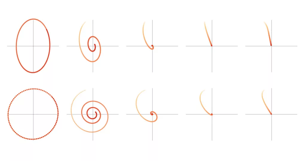
We can break this equation apart to see how each component affects the dynamics of the system. Here we plot, for

$150$

This system is best imagined as a weight suspended on a spring. We pull the weight down by one unit, and we study the path it follows as it returns to equilibrium. In the analogy, the spring is the source of our external force

$lambda_ix^k_i$

$x^k_i$

$y^k_i$

$beta$

The critical value of

$beta = (1 – sqrt{alpha lambda_i})^2$

$i$

$1 – sqrt{alphalambda_i}.$

$1-alphalambda_i$

$i^{th}$

$alpha$

Optimal parameters

To get a global convergence rate, we must optimize over both

$alpha$

$beta$

$alpha = left(frac{2}{sqrt{lambda_{1}}+sqrt{lambda_{n}}}right)^{2} quad beta = left(frac{sqrt{lambda_{n}}-sqrt{lambda_{1}}}{sqrt{lambda_{n}}+sqrt{lambda_{1}}}right)^{2}$

$frac{sqrt{kappa}-1}{sqrt{kappa}+1}$

Convergence rate, Momentum

$frac{kappa-1}{kappa+1}$

Convergence rate, Gradient Descent

With barely a modicum of extra effort, we have essentially square rooted the condition number! These gains, in principle, require explicit knowledge of

$lambda_1$

$lambda_n$

$alpha$

$1$

$beta$

$1$

$alpha$

We can do the same decomposition here with momentum, with eigenvalues

$lambda_1=0.01$

$lambda_2=0.1$

$lambda_3=1$

$f(w^k) – f(w^star)$

Note that the optimal parameters do not necessarily imply the fastest convergence, though, only the fastest asymptotic convergence rate.

Step-size α =

Momentum β =

While the loss function of gradient descent had a graceful, monotonic curve, optimization with momentum displays clear oscillations. These ripples are not restricted to quadratics, and occur in all kinds of functions in practice. They are not cause for alarm, but are an indication that extra tuning of the hyperparameters is required.

Example: The Colorization Problem

Let’s look at how momentum accelerates convergence with a concrete example. On a grid of pixels let

$G$

$E$

$D$

$text{minimize}$

$qquad frac{1}{2} sum_{iin D} (w_i – 1)^2$

The colorizer pulls distinguished pixels towards 1

$+$

$frac{1}{2} sum_{i,jin E} (w_i – w_j)^2.$

The smoother spreads out the color

The optimal solution to this problem is a vector of all

$1$

$w_{i}^{k+1}=w_{i}^{k}-alphasum_{jin N}(w_{i}^{k}-w_{j}^{k})-begin{cases} alpha(w_{i}^{k}-1) & iin D\ 0 & inotin D end{cases}$

This kind of local averaging is effective at smoothing out local variations in the pixels, but poor at taking advantage of global structure. The updates are akin to a drop of ink, diffusing through water. Movement towards equilibrium is made only through local corrections and so, left undisturbed, its march towards the solution is slow and laborious. Fortunately, momentum speeds things up significantly.

The eigenvectors of the colorization problem form a generalized Fourier basis for

$R^n$

In vectorized form, the colorization problem is

$text{minimize}$

The smoother’s quadratic form is the Graph Laplacian

$frac{1}{2}sum_{iin D}left(x^{T}e_{i}e_{i}^{T}x-e_{i}^{T}xright)$

$+$

$frac{1}{2}x^{T}L_{G}x$

And the colorizer is a small low rank correction with a linear term.

$e_i$

$i^{th}$

The Laplacian matrix,

$L_G$

Small world graphs, like expanders and dense graphs, have excellent conditioning

The conditioning of grids improves with its dimensionality.

And long, wiry graphs, like paths, condition poorly.

These observations carry through to the colorization problem, and the intuition behind it should be clear. Well connected graphs allow rapid diffusion of information through the edges, while graphs with poor connectivity do not. And this principle, taken to the extreme, furnishes a class of functions so hard to optimize they reveal the limits of first order optimization.

The Limits of Descent

Let’s take a step back. We have, with a clever trick, improved the convergence of gradient descent by a quadratic factor with the introduction of a single auxiliary sequence. But is this the best we can do? Could we improve convergence even more with two sequences? Could one perhaps choose the

$alpha$

$beta$

Unfortunately, while improvements to the momentum algorithm do exist, they all run into a certain, critical, almost inescapable lower bound.

Adventures in Algorithmic Space

To understand the limits of what we can do, we must first formally define the algorithmic space in which we are searching. Here’s one possible definition. The observation we will make is that both gradient descent and momentum can be “unrolled”. Indeed, since

$begin{array}{lll} w^{1} & != & !w^{0} ~-~ alphanabla f(w^{0})\[0.35em] w^{2} & != & !w^{1} ~-~ alphanabla f(w^{1})\[0.35em] & != & !w^{0} ~-~ alphanabla f(w^{0}) ~-~ alphanabla f(w^{1})\[0.35em] & ~ !vdots \ w^{k+1} & != & !w^{0} ~-~ alphanabla f(w^{0}) ~-~~~~ cdotscdots ~~~~-~ alphanabla f(w^{k}) end{array}$

$w^{k+1} ~~=~~ w^{0} ~-~ alphasum_i^knabla f(w^{i}).$

A similar trick can be done with momentum:

$w^{k+1} ~~=~~ w^{0} ~+~ alphasum_i^kfrac{(1-beta^{k+1-i})}{1-beta}nabla f(w^i).$

In fact, all manner of first order algorithms, including the Conjugate Gradient algorithm, AdaMax, Averaged Gradient and more, can be written (though not quite so neatly) in this unrolled form. Therefore the class of algorithms for which

$w^{k+1} ~~=~~ w^{0} ~+~ sum_{i}^{k}gamma_{i}^{k}nabla f(w^{i}) qquad text{ for some } gamma_{i}^{k}$

contains momentum, gradient descent and a whole bunch of other algorithms you might dream up. This is what is assumed in Assumption 2.1.4[5] of Nesterov. But let’s push this even further, and expand this class to allow different step-sizes for different directions.

$w^{k+1} ~~=~~ w^{0} ~+~ sum_{i}^{k}Gamma_{i}^{k}nabla f(w^{i}) quad text{ for some diagonal matrix } Gamma_{i}^{k} .$

This class of methods covers most of the popular algorithms for training neural networks, including ADAM and AdaGrad. We shall refer to this class of methods as “Linear First Order Methods”, and we will show a single function all these methods ultimately fail on.

The Resisting Oracle

Earlier, when we talked about the colorizer problem, we observed that wiry graphs cause bad conditioning in our optimization problem. Taking this to its extreme, we can look at a graph consisting of a single path — a function so badly conditioned that Nesterov called a variant of it “the worst function in the world”. The function follows the same structure as the colorizer problem, and we shall call this the Convex Rosenbrock,

$f^n(w)$

$=$

with a colorizer of one node

$frac{1}{2}left(w_{1}-1right)^{2}$

$+$

$frac{1}{2}sum_{i=1}^{n}(w_{i}-w_{i+1})^{2}$

strong couplings of adjacent nodes in the path,

$+$

$frac{2}{kappa-1}|w|^{2}.$

and a small regularization term.

The optimal solution of this problem is

$w_{i}^{star}=left(frac{sqrt{kappa}-1}{sqrt{kappa}+1}right)^{i}$

and the condition number of the problem

$f^n$

$kappa$

$n$

$w^0 = 0$

Step-size α =

Momentum β =

Here we see the first 50 iterates of momentum on the Convex Rosenbrock for

$n=25$

This triangle is a “dead zone” of our iterates. The iterates are always 0, no matter what the parameters.

The remaining expanding space is the “light cone” of our iterate’s influence. Momentum does very well here with the optimal parameters.

Error

Weights

The observations made in the above diagram are true for any Linear First Order algorithm. Let us prove this. First observe that each component of the gradient depends only on the values directly before and after it:

$nabla f(x)_{i}=2w_{i}-w_{i-1}-w_{i+1} +frac{4}{kappa-1} w_{i}, qquad i neq 1.$

Therefore the fact we start at 0 guarantees that that component must remain stoically there till an element either before or after it turns nonzero. And therefore, by induction, for any linear first order algorithm,

$begin{array}{lllllllll} w^{0} & = & [~~0, & 0, & 0, & ldots & 0, & 0, & ldots & 0~]\[0.35em] w^{1} & = & [~w_{1}^{1}, & 0, & 0, & ldots & 0, & 0, & ldots & 0~]\[0.35em] w^{2} & = & [~w_{1}^{2}, & w_{2}^{2}, & 0, & ldots & 0, & 0, & ldots & 0~]\[0.35em] & ~ vdots \ w^{k} & = & [~w_{1}^{k}, & w_{2}^{k}, & w_{3}^{k}, & ldots & w_{k}^{k}, & 0, & ldots & 0~].\ end{array}$

Think of this restriction as a “speed of light” of information transfer. Error signals will take at least

$k$

$w_0$

$w_k$

$begin{aligned} |w^{k}-w^{star}|_{infty}&geqmax_{igeq k+1}{|w_{i}^{star}|}\[0.9em]&=left(frac{sqrt{kappa}-1}{sqrt{kappa}+1}right)^{k+1}\[0.9em]&=left(frac{sqrt{kappa}-1}{sqrt{kappa}+1}right)^{k}|w^{0}-w^{star}|_{infty}. end{aligned}$

$n$

$f^n$

$kappa$

Like many such lower bounds, this result must not be taken literally, but spiritually. It, perhaps, gives a sense of closure and finality to our investigation. But this is not the final word on first order optimization. This lower bound does not preclude the possibility, for example, of reformulating the problem to change the condition number itself! There is still much room for speedups, if you understand the right places to look.

Momentum with Stochastic Gradients

There is a final point worth addressing. All the discussion above assumes access to the true gradient — a luxury seldom afforded in modern machine learning. Computing the exact gradient requires a full pass over all the data, the cost of which can be prohibitively expensive. Instead, randomized approximations of the gradient, like minibatch sampling, are often used as a plug-in replacement of

$nabla f(w)$

the true gradient

$+$

$text{error}(w).$

and an approximation error.
If the estimator is unbiased e.g.

$mathbf{E}[text{error}(w)] = 0$

It is helpful to think of our approximate gradient as the injection of a special kind of noise into our iteration. And using the machinery developed in the previous sections, we can deal with this extra term directly. On a quadratic, the error term cleaves cleanly into a separate term, where¹⁰

$left(begin{array}{c} y_{i}^{k}\ x_{i}^{k} end{array}right)$

the noisy iterates are a sum of

$=$

$R^{k}left(begin{array}{c} y_{i}^{0}\ x_{i}^{0} end{array}right)$

the noiseless, deterministic iterates and

$+$

$epsilon^k_i sum_{j=1}^{k}R^{k-j}left(begin{array}{c} 1\ -alpha end{array}right)$

a decaying sum of the errors, where

$epsilon^k = Q cdot text{error}(w^k)$

The error term,

$epsilon^k$

$w^k$

We decompose the expected value of the objective value

$mathbf{E} f(w) – f(w^star)$

The small black dots are a single run of stochastic gradient

Step-size α =

Momentum β =

As[1] observes, the optimization has two phases. In the initial transient phase the magnitude of the noise is smaller than the magnitude of the gradient, and Momentum still makes good progress. In the second, stochastic phase, the noise overwhelms the gradient, and momentum is less effective.

Note that there are a set of unfortunate tradeoffs which seem to pit the two components of error against each other. Lowering the step-size, for example, decreases the stochastic error, but also slows down the rate of convergence. And increasing momentum, contrary to popular belief, causes the errors to compound. Despite these undesirable properties, stochastic gradient descent with momentum has still been shown to have competitive performance on neural networks. As[1] has observed, the transient phase seems to matter more than the fine-tuning phase in machine learning. And in fact, it has been recently suggested[12] that this noise is a good thing — it acts as a implicit regularizer, which, like early stopping, prevents overfitting in the fine-tuning phase of optimization.

Onwards and Downwards

The study of acceleration is seeing a small revival within the optimization community. If the ideas in this article excite you, you may wish to read[13], which fully explores the idea of momentum as the discretization of a certain differential equation. But other, less physical, interpretations exist. There is an algebraic interpretation of momentum in terms of approximating polynomials[3, 14]. Geometric interpretations are emerging[15, 16], connecting momentum to older methods, like the Ellipsoid method. And finally, there are interpretations relating momentum to duality[17], perhaps providing a clue as how to accelerate second order methods and Quasi Newton (for a first step, see[18]). But like the proverbial blind men feeling an elephant, momentum seems like something bigger than the sum of its parts. One day, hopefully soon, the many perspectives will converge into a satisfying whole.

Acknowledgments

I am deeply indebted to the editorial contributions of Shan Carter and Chris Olah, without which this article would be greatly impoverished. Shan Carter provided complete redesigns of many of my original interactive widgets, a visual coherence for all the figures, and valuable optimizations to the page’s performance. Chris Olah provided impeccable editorial feedback at all levels of detail and abstraction – from the structure of the content, to the alignment of equations.

I am also grateful to Michael Nielsen for providing the title of this article, which really tied the article together. Marcos Ginestra provided editorial input for the earliest drafts of this article, and spiritual encouragement when I needed it the most. And my gratitude extends to my reviewers, Matt Hoffman and Anonymous Reviewer B for their astute observations and criticism. I would like to thank Reviewer B, in particular, for pointing out two non-trivial errors in the original manuscript (discussion here). The contour plotting library for the hero visualization is the joint work of Ben Frederickson, Jeff Heer and Mike Bostock.

Many thanks to the numerous pull requests and issues filed on github. Thanks in particular, to Osemwaro Pedro for spotting an off by one error in one of the equations. And also to Dan Schmidt who did an editing pass over the whole project, correcting numerous typographical and grammatical errors.

Discussion and Review

Reviewer A – Matt Hoffman
Reviewer B – Anonymous
Discussion with User derifatives

Footnotes

It is possible, however, to construct very specific counterexamples where momentum does not converge, even on convex functions. See[4] for a counterexample.
In Tikhonov Regression we add a quadratic penalty to the regression, minimizing
$text{minimize}qquadtfrac{1}{2}|Zw-d|^{2}+frac{eta}{2}|w|^{2}=tfrac{1}{2}w^{T}(Z^{T}Z+eta I)w-(Zd)^{T}w$
$Z^{T}Z=Q text{diag}(Lambda_{1},ldots,Lambda_{n}) Q^T$
$(Z^{T}Z+eta I)^{-1}(Zd)=Q text{diag}left(frac{1}{lambda_{1}+eta},cdots,frac{1}{lambda_{n}+eta}right)Q^T(Zd)$
$text{Tikhonov Regularized } lambda_i = frac{1}{lambda_{i}+eta}=frac{1}{lambda_{i}}left(1-left(1+lambda_{i}/etaright)^{-1}right).$
$text{ Gradient Descent Regularized } lambda_i = frac{1}{lambda_i} left( 1-left(1-alphalambda_{i}right)^{k} right)$
This is true as we can write updates in matrix form as
$left(!!begin{array}{cc} 1 & 0\ alpha & 1 end{array}!!right)Bigg(!!begin{array}{c} y_{i}^{k+1}\ x_{i}^{k+1} end{array}!!Bigg)=left(!!begin{array}{cc} beta & lambda_{i}\ 0 & 1 end{array}!!right)left(!!begin{array}{c} y_{i}^{k}\ x_{i}^{k} end{array}!!right)$
which implies, by inverting the matrix on the left,
$Bigg(!!begin{array}{c} y_{i}^{k+1}\ x_{i}^{k+1} end{array}!!Bigg)=left(!!begin{array}{cc} beta & lambda_{i}\ -alphabeta & 1-alphalambda_{i} end{array}!!right)left(!!begin{array}{c} y_{i}^{k}\ x_{i}^{k} end{array}!!right)=R^{k+1}left(!!begin{array}{c} x_{i}^{0}\ y_{i}^{0} end{array}!!right)$
We can write out the convergence rates explicitly. The eigenvalues are
$begin{aligned} sigma_{1} & =frac{1}{2}left(1-alphalambda+beta+sqrt{(-alphalambda+beta+1)^{2}-4beta}right)\[0.6em] sigma_{2} & =frac{1}{2}left(1-alphalambda+beta-sqrt{(-alphalambda+beta+1)^{2}-4beta}right) end{aligned}$
$(-alphalambda+beta+1)^{2}-4beta<0$
$begin{aligned} |sigma_{1}|=|sigma_{2}| & =sqrt{(1-alphalambda+beta)^{2}+|(-alphalambda+beta+1)^{2}-4beta|}=2sqrt{beta} end{aligned}$
$alphalambda$
$max{|sigma_{1}|,|sigma_{2}|}=tfrac{1}{2}maxleft{ |1-alphalambda_{i}+betapmsqrt{(1-alphalambda_{i}+beta)^{2}-4beta}|right}$
This can be derived by reducing the inequalities for all 4 + 1 cases in the explicit form of the convergence rate above.
We must optimize over
$min_{alpha,beta}maxleft{ bigg| ! left(begin{array}{cc} beta & lambda_{i}\ -alphabeta & 1-alphalambda_{i} end{array}right) ! bigg|,ldots,bigg| ! left(begin{array}{cc} beta & lambda_{n}\ -alphabeta & 1-alphalambda_{n} end{array}right)! bigg|right}.$
$|cdot |$
The above optimization problem is bounded from below by
$0$
$1$
This can be written explicitly as
$[L_{G}]_{ij}=begin{cases} text{degree of vertex }i & i=j\ -1 & ineq j,(i,j)text{ or }(j,i)in E\ 0 & text{otherwise} end{cases}$
We use the infinity norm to measure our error, similar results can be derived for the 1 and 2 norms.
The momentum iterations are
$begin{aligned} z^{k+1}&=beta z^{k}+ A w^{k} + text{error}(w^k) \[0.4em] w^{k+1}&=w^{k}-alpha z^{k+1}. end{aligned}$
$left(!!begin{array}{cc} 1 & 0\ alpha & 1 end{array}!!right)Bigg(!!begin{array}{c} y_{i}^{k+1}\ x_{i}^{k+1} end{array}!!Bigg)=left(!!begin{array}{cc} beta & lambda_{i}\ 0 & 1 end{array}!!right)left(!!begin{array}{c} y_{i}^{k}\ x_{i}^{k} end{array}!!right)+left(!!begin{array}{c} epsilon_{i}^{k}\ 0 end{array}!!right)$
$2 times 2$
On the 1D function
$f(x)=frac{lambda}{2}x^{2}$
$begin{aligned} mathbf{E}f(x^{k})&=frac{lambda}{2}mathbf{E}[(x^{k})^{2}]\&=frac{lambda}{2}mathbf{E}left(e_{2}^{T}R^{k}left(begin{array}{c} y^{0}\ x^{0} end{array}right)+epsilon^{k}e_{2}^{T}sum_{i=1}^{k}R^{k-i}left(begin{array}{c} 1\ -alpha end{array}right)right)^{2}\&=frac{lambda}{2}e_{2}^{T}R^{k}left(begin{array}{c} y^{0}\ x^{0} end{array}right)+frac{lambda}{2}mathbf{E}left(epsilon^{k}e_{2}^{T}sum_{i=1}^{k}R^{k-i}left(begin{array}{c} 1\ -alpha end{array}right)right)^{2}\&=frac{lambda}{2}e_{2}^{T}R^{k}left(begin{array}{c} y^{0}\ x^{0} end{array}right)+frac{lambda}{2}mathbf{E}[epsilon^{k}],cdot,sum_{i=1}^{k}left(e_{2}^{T}R^{k-i}left(begin{array}{c} 1\ -alpha end{array}right)right)^{2}\&=frac{lambda}{2}e_{2}^{T}R^{k}left(begin{array}{c} y^{0}\ x^{0} end{array}right)+frac{lambdamathbf{E}[epsilon^{k}}{2}cdotsum_{i=1}^{k}gamma_{i}^{2}, qquad gamma_i = e_{2}^{T}R^{k-i}left(begin{array}{c} 1\ -alpha end{array}right) end{aligned}$
$mathbf{E} epsilon^k = 0$

References

On the importance of initialization and momentum in deep learning. [PDF]
Sutskever, I., Martens, J., Dahl, G.E. and Hinton, G.E., 2013. ICML (3), Vol 28, pp. 1139—1147.
Some methods of speeding up the convergence of iteration methods [PDF]
Polyak, B.T., 1964. USSR Computational Mathematics and Mathematical Physics, Vol 4(5), pp. 1—17. Elsevier. DOI: 10.1016/0041-5553(64)90137-5
Theory of gradient methods
Rutishauser, H., 1959. Refined iterative methods for computation of the solution and the eigenvalues of self-adjoint boundary value problems, pp. 24—49. Springer. DOI: 10.1007/978-3-0348-7224-9_2
Analysis and design of optimization algorithms via integral quadratic constraints [PDF]
Lessard, L., Recht, B. and Packard, A., 2016. SIAM Journal on Optimization, Vol 26(1), pp. 57—95. SIAM.
Introductory lectures on convex optimization: A basic course
Nesterov, Y., 2013. , Vol 87. Springer Science & Business Media. DOI: 10.1007/978-1-4419-8853-9
Natural gradient works efficiently in learning http://distill.pub/2017/momentum
Amari, S., 1998. Neural computation, Vol 10(2), pp. 251—276. MIT Press. DOI: 10.1162/089976698300017746
Deep Learning, NIPS′2015 Tutorial [PDF]
Hinton, G., Bengio, Y. and LeCun, Y., 2015.
Adaptive restart for accelerated gradient schemes [PDF]
O’Donoghue, B. and Candes, E., 2015. Foundations of computational mathematics, Vol 15(3), pp. 715—732. Springer. DOI: 10.1007/s10208-013-9150-3
The Nth Power of a 2×2 Matrix. [PDF]
Williams, K., 1992. Mathematics Magazine, Vol 65(5), pp. 336. MAA. DOI: 10.2307/2691246
From Averaging to Acceleration, There is Only a Step-size. [PDF]
Flammarion, N. and Bach, F.R., 2015. COLT, pp. 658—695.
On the momentum term in gradient descent learning algorithms [PDF]
Qian, N., 1999. Neural networks, Vol 12(1), pp. 145—151. Elsevier. DOI: 10.1016/s0893-6080(98)00116-6
Understanding deep learning requires rethinking generalization [PDF]
Zhang, C., Bengio, S., Hardt, M., Recht, B. and Vinyals, O., 2016. arXiv preprint arXiv:1611.03530.
A differential equation for modeling Nesterov’s accelerated gradient method: Theory and insights [PDF]
Su, W., Boyd, S. and Candes, E., 2014. Advances in Neural Information Processing Systems, pp. 2510—2518.
The Zen of Gradient Descent [HTML]
Hardt, M., 2013.
A geometric alternative to Nesterov’s accelerated gradient descent [PDF]
Bubeck, S., Lee, Y.T. and Singh, M., 2015. arXiv preprint arXiv:1506.08187.
An optimal first order method based on optimal quadratic averaging [PDF]
Drusvyatskiy, D., Fazel, M. and Roy, S., 2016. arXiv preprint arXiv:1604.06543.
Linear coupling: An ultimate unification of gradient and mirror descent [PDF]
Allen-Zhu, Z. and Orecchia, L., 2014. arXiv preprint arXiv:1407.1537.
Accelerating the cubic regularization of Newton’s method on convex problems [PDF]
Nesterov, Y., 2008. Mathematical Programming, Vol 112(1), pp. 159—181. Springer. DOI: 10.1007/s10107-006-0089-x

Updates and Corrections

View all changes to this article since it was first published. If you see a mistake or want to suggest a change, please create an issue on GitHub.

Citations and Reuse

Diagrams and text are licensed under Creative Commons Attribution CC-BY 2.0, unless noted otherwise, with the source available on GitHub. The figures that have been reused from other sources don’t fall under this license and can be recognized by a note in their caption: “Figure from …”.

For attribution in academic contexts, please cite this work as

Goh, "Why Momentum Really Works", Distill, 2017. http://doi.org/10.23915/distill.00006

BibTeX citation

@article{goh2017why,
  author = {Goh, Gabriel},
  title = {Why Momentum Really Works},
  journal = {Distill},
  year = {2017},
  url = {http://distill.pub/2017/momentum},
  doi = {10.23915/distill.00006}
}

Source link