Even if you have spent some time reading about machine learning, chances are that you have never heard of Gaussian processes.
And if you have, rehearsing the basics is always a good way to refresh your memory.
With this blog post we want to give an introduction to Gaussian processes and make the mathematical intuition behind them more approachable.

Gaussian processes are a powerful tool in the machine learning toolbox.
They allow us to make predictions about our data by incorporating prior knowledge.
Their most obvious area of application is fitting a function to the data.
This is called regression and is used, for example, in robotics or time series forecasting.
But Gaussian processes are not limited to regression — they can also be extended to classification and clustering tasks.

For a given set of training points, there are potentially infinitely many functions that fit the data.
Gaussian processes offer an elegant solution to this problem by assigning a probability to each of these functions.
The mean of this probability distribution then represents the most probable characterization of the data.
Furthermore, using a probabilistic approach allows us to incorporate the confidence of the prediction into the regression result.

We will first explore the mathematical foundation that Gaussian processes are built on — we invite you to follow along using the interactive figures and hands-on examples.
They help to explain the impact of individual components, and show the flexibility of Gaussian processes.
After following this article we hope that you will have a visual intuition on how Gaussian processes work and how you can configure them for different types of data.

Multivariate Gaussian distributions

Before we can explore Gaussian processes, we need to understand the mathematical concepts they are based on.
As the name suggests, the Gaussian distribution (which is often also referred to as normal distribution) is the basic building block of Gaussian processes.
In particular, we are interested in the multivariate case of this distribution, where each random variable is distributed normally and their joint distribution is also Gaussian.
The multivariate Gaussian distribution is defined by a mean vector $mu$ and a covariance matrix $Sigma$.
You can see an interactive example of such distributions in the figure below.

The mean vector $mu$ describes the expected value of the distribution.
Each of its components describes the mean of the corresponding dimension.
$Sigma$ models the variance along each dimension and determines how the different random variables are correlated.
The covariance matrix is always symmetric and positive semi-definite.
The diagonal of $Sigma$ consists of the variance $sigma_i^2$

$X = begin{bmatrix} X_1 \ X_2 \ vdots \ X_n end{bmatrix} sim mathcal{N}(mu, Sigma)$

We say $X$ follows a normal distribution. The covariance matrix $Sigma$ describes the shape of the distribution. It is defined in terms of the expected value $E$:

$Sigma = text{Cov}(X_i, X_j) = E left[ (X_i – mu_i)(X_j – mu_j)^T right]$

Visually, the distribution is centered around the mean and the covariance matrix defines its shape. The following figure shows the influence of these parameters on a two-dimensional Gaussian distribution. The variances for each random variable are on the diagonal of the covariance matrix, while the other values show the covariance between them.

Gaussian distributions are widely used to model the real world.
For example, we can employ them to describe errors of measurements or phenomena under the assumptions of the central limit theorem

One of the implications of this theorem is that a collection of independent, identically distributed random variables with finite variance have a mean that is distributed normally.
A good introduction to the central limit theorem is given by this video from Khan Academy.
.
In the next section we will take a closer look at how to manipulate Gaussian distributions and extract useful information from them.

Marginalization and Conditioning

Gaussian distributions have the nice algebraic property of being closed under conditioning and marginalization.
Being closed under conditioning and marginalization means that the resulting distributions from these operations are also Gaussian, which makes many problems in statistics and machine learning tractable.
In the following we will take a closer look at both of these operations, as they are the foundation for Gaussian processes.

Marginalization and conditioning both work on subsets of the original distribution and we will use the following notation:

$P_{X,Y} = begin{bmatrix} X \ Y end{bmatrix} sim mathcal{N}(mu, Sigma) = mathcal{N} left( begin{bmatrix} mu_X \ mu_Y end{bmatrix}, begin{bmatrix} Sigma_{XX} , Sigma_{XY} \ Sigma_{YX} , Sigma_{YY} end{bmatrix} right)$

With $X$ and $Y$ representing subsets of original random variables.

Through marginalization we can extract partial information from multivariate probability distributions. In particular, given a normal probability distribution $P(X,Y)$ over vectors of random variables $X$ and $Y$, we can determine their marginalized probability distributions in the following way:

$begin{aligned} X &sim mathcal{N}(mu_X, Sigma_{XX}) \ Y &sim mathcal{N}(mu_Y, Sigma_{YY}) end{aligned}$

The interpretation of this equation is that each partition $X$ and $Y$ only depends on its corresponding entries in $mu$ and $Sigma$.
To marginalize out a random variable from a Gaussian distribution we can simply drop the variables from $mu$ and $Sigma$.

$p_X(x) = int_y p_{X,Y}(x,y)dy = int_y p_{X|Y}(x|y) p_Y(y) dy$

The way to interpret this equation is that if we are interested in the probability density of
$X = x$, we need to consider all possible outcomes of
$Y$ that can jointly lead to the result
The corresponding Wikipedia
article has a good description of the marginal distribution, including several examples.
.

Another important operation for Gaussian processes is conditioning.
It is used to determine the probability of one variable depending on another variable.
Similar to marginalization, this operation is also closed and yields a modified Gaussian distribution.
This operation is the cornerstone of Gaussian processes since it allows Bayesian inference, which we will talk about in the next section.
Conditioning is defined by:

$begin{aligned} X|Y &sim mathcal{N}(:mu_X + Sigma_{XY}Sigma_{YY}^{-1}(Y – mu_Y),: Sigma_{XX}-Sigma_{XY}Sigma_{YY}^{-1}Sigma_{YX}:) \ Y|X &sim mathcal{N}(:mu_Y + Sigma_{YX}Sigma_{XX}^{-1}(X – mu_X),: Sigma_{YY}-Sigma_{YX}Sigma_{XX}^{-1}Sigma_{XY}:) \ end{aligned}$

Note that the new mean only depends on the conditioned variable, while the covariance matrix is independent from this variable.

Now that we have worked through the necessary equations, we will think about how we can understand the two operations visually.
While marginalization and conditioning can be applied to multivariate distributions of many dimensions, it makes sense to consider the two-dimensional case as shown in the following figure.
Marginalization can be seen as integrating along one of the dimensions of the Gaussian distribution, which is in line with the general definition of the marginal distribution.
Conditioning also has a nice geometric interpretation — we can imagine it as making a cut through the multivariate distribution, yielding a new Gaussian distribution with fewer dimensions.

Gaussian Processes

Now that we have recalled some of the basic properties of multivariate Gaussian distributions, we will combine them together to define Gaussian processes, and show how they can be used to tackle regression problems.

First, we will move from the continuous view to the discrete representation of a function:
rather than finding an implicit function, we are interested in predicting the function values at concrete points, which we call test points $X$.
So how do we derive this functional view from the multivariate normal distributions that we have considered so far?
Stochastic processes, such as Gaussian processes, are essentially a set of random variables.
In addition, each of these random variables has a corresponding index $i$.
We will use this index to refer to the $i$-th dimension of our $n$-dimensional multivariate distributions.
The following figure shows an example of this for two dimensions:

Now, the goal of Gaussian processes is to learn this underlying distribution from training data.
Respective to the test data $X$, we will denote the training data as $Y$.
As we have mentioned before, the key idea of Gaussian processes is to model the underlying distribution of $X$ together with $Y$ as a multivariate normal distribution.
That means that the joint probability distribution $P_{X,Y}$

In order to perform regression on the training data, we will treat this problem as Bayesian inference.
The essential idea of Bayesian inference is to update the current hypothesis as new information becomes available.
In the case of Gaussian processes, this information is the training data.
Thus, we are interested in the conditional probability $P_{X|Y}$

Now that we have the basic framework of Gaussian processes together, there is only one thing missing:
how do we set up this distribution and define the mean $mu$ and the covariance matrix $Sigma$?
The covariance matrix $Sigma$ is determined by its covariance function $k$, which is often also called the kernel of the Gaussian process.
We will talk about this in detail in the next section.
But before we come to this, let us reflect on how we can use multivariate Gaussian distributions to estimate function values.
The following figure shows an example of this using ten test points at which we want to predict our function:

In Gaussian processes we treat each test point as a random variable.
A multivariate Gaussian distribution has the same number of dimensions as the number of random variables.
Since we want to predict the function values at
$|X|=N$
test points, the corresponding multivariate Gaussian distribution is also
$N$
-dimensional.
Making a prediction using a Gaussian process ultimately boils down to drawing samples from this distribution.
We then interpret the $i$-th component of the resulting vector as the function value corresponding to the $i$-th test point.

Kernels

Recall that in order to set up our distribution, we need to define $mu$ and $Sigma$.
In Gaussian processes it is often assumed that $mu = 0$, which simplifies the necessary equations for conditioning.
We can always assume such a distribution, even if $mu neq 0$, and add $mu$ back to the resulting function values after the prediction step.
This process is also called centering of the data.
So configuring $mu$ is straight forward — it gets more interesting when we look at the other parameter of the distribution.

The clever step of Gaussian processes is how we set up the covariance matrix $Sigma$.
The covariance matrix will not only describe the shape of our distribution, but ultimately determines the characteristics of the function that we want to predict.
We generate the covariance matrix by evaluating the kernel $k$, which is often also called covariance function, pairwise on all the points.
The kernel receives two points $t,t’ in mathbb{R}^n$

$k: mathbb{R}^n times mathbb{R}^n rightarrow mathbb{R},quad Sigma = text{Cov}(X,X’) = k(t,t’)$

We evaluate this function for each pairwise combination of the test points to retrieve the covariance matrix.
This step is also depicted in the figure above.
In order to get a better intuition for the role of the kernel, let’s think about what the entries in the covariance matrix describe.
The entry $Sigma_{ij}$

Kernels are widely used in machine learning, for example in support vector machines.
The reason for this is that they allow similarity measures that go far beyond the standard euclidean distance ($L2$-distance).
Many of these kernels conceptually embed the input points into a higher dimensional space in which they then measure the similarityIf the kernel follows Mercer’s theorem it can be used to define a Hilbert space. More information on this can be found on Wikipedia..
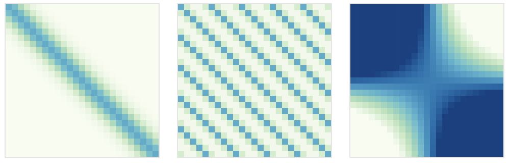
The following figure shows examples of some common kernels for Gaussian processes.
For each kernel, the covariance matrix has been created from $N=25$ linearly-spaced values ranging from $[-5,5]$. Each entry in the matrix shows the covariance between points in the range of $[0,1]$.

Kernels can be separated into stationary and non-stationary kernels. Stationary kernels, such
as the RBF kernel or the periodic kernel, are functions invariant to translations, and the covariance of two points is only
dependent on their relative position. Non-stationary kernels, such as the linear kernel, do not have this
constraint and depend on an absolute location. The stationary nature of the RBF kernel can be observed in the
banding around the diagonal of its covariance matrix (as shown in this figure). Increasing the length parameter increases the banding, as
points further away from each other become more correlated. For the periodic kernel, we have an additional parameter
$P$ that determines the periodicity, which controls the distance between each repetition of the function.
In contrast, the parameter $C$ of the linear kernel allows us to change the point on which all functions hinge.

There are many more kernels that can describe different classes of functions, which can be used to model the desired shape of the function.
A good overview of different kernels is given by Duvenaud.
It is also possible to combine several kernels — but we will get to this later.

Prior Distribution

We will now shift our focus back to the original task of regression.
As we have mentioned earlier, Gaussian processes define a probability distribution over possible functions.
In this figure above, we show this connection:
each sample of our multivariate normal distribution represents one realization of our function values.
Because this distribution is a multivariate Gaussian distribution, the distribution of functions is normal.
Recall that we usually assume $mu=0$.
For now, let’s consider the case where we have not yet observed any training data.
In the context of Bayesian inference, this is called the prior distribution $P_X$

If we have not yet observed any training examples, this distribution revolves around $mu=0$, according to our original assumption.
The prior distribution will have the same dimensionality as the number of test points $N = |X|$.
We will use the kernel to set up the covariance matrix, which has the dimensions $N times N$.

In the previous section we have looked at examples of different kernels.
The kernel is used to define the entries of the covariance matrix.
Consequently, the covariance matrix determines which type of functions from the space of all possible functions are more probable.
As the prior distribution does not yet contain any additional information, it is perfect to visualize the influence of the kernel on the distribution of functions.
The following figure shows samples of potential functions from prior distributions that were created using different kernels:

Adjusting the parameters allows you to control the shape of the resulting functions.
This also varies the confidence of the prediction.
When decreasing the variance $sigma$, a common parameter for all kernels, sampled functions are more concentrated around the mean $mu$.
For the Linear kernel, setting the variance $sigma_b=0$

Posterior Distribution

So what happens if we observe training data?
Let’s get back to the model of Bayesian inference, which states that we can incorporate this additional information into our model, yielding the posterior distribution $P_{X|Y}$

First, we form the joint distribution $P_{X,Y}$

For the next step we need one operation on Gaussian distributions that we have defined earlier.
Using conditioning we can find $P_{X|Y}$

As mentioned before, the conditional distribution $P_{X|Y}$

$Y = f(X) + epsilon$

We do this by slightly modifying the setup of the joint distribution $P_{X,Y}$

$P_{X,Y} = begin{bmatrix} X \ Y end{bmatrix} sim mathcal{N}(0, Sigma) = mathcal{N} left( begin{bmatrix} 0 \ 0 end{bmatrix}, begin{bmatrix} Sigma_{XX} & Sigma_{XY} \ Sigma_{YX} & Sigma_{YY}+psi^2I end{bmatrix} right)$

Again, we can use conditioning to derive the predictive distribution $P_{X|Y}$

Analogous to the prior distribution, we could obtain a prediction for our function values by sampling from this distribution.
But, since sampling involves randomness, the resulting fit to the data would not be deterministic and our prediction could end up being an outlier.
In order to make a more meaningful prediction we can use the other basic operation of Gaussian distributions.

Through the marginalization of each random variable, we can extract the respective mean function value $mu’_i$

The following figure shows an example of the conditional distribution.
At first, no training points have been observed.
Accordingly, the mean prediction remains at $0$ and the standard deviation is the same for each test point.
By hovering over the covariance matrix you can see the influence of each point on the current test point.
As long as no training points have been observed, the influence of neighboring points is limited locally.

The training points can be activated by clicking on them, which leads to a constrained distribution.
This change is reflected in the entries of the covariance matrix, and leads to an adjustment of the mean and the standard deviation of the predicted function.
As we would expect, the uncertainty of the prediction is small in regions close to the training data and grows as we move further away from those points.

In the constrained covariance matrix, we can see that the correlation of neighbouring points is affected by the
training data.
If a predicted point lies on the training data, there is no correlation with other points.
Therefore, the function must pass directly through it.
Predicted values further away are also affected by the training data — proportional to their distance.

Combining different kernels

As described earlier, the power of Gaussian processes lies in the choice of the kernel function.
This property allows experts to introduce domain knowledge into the process and lends Gaussian processes their flexibility to capture trends in the training data.
For example, by choosing a suitable bandwidth for the RBF kernel, we can control how smooth the resulting function will be.

A big benefit that kernels provide is that they can be combined together, resulting in a more specialized kernel.
The decision which kernel to use is highly dependent on prior knowledge about the data, e.g. if certain characteristics are expected.
Examples for this would be stationary nature, or global trends and patterns.
As introduced in the section on kernels, stationary means that a kernel is translation invariant and therefore not dependent on the index $i$.
This also means that we cannot model global trends using a strictly stationary kernel.
Remember that the covariance matrix of Gaussian processes has to be positive semi-definite.
When choosing the optimal kernel combinations, all methods that preserve this property are allowed.
The most common kernel combinations would be addition and multiplication.

Let’s consider two kernels, a linear kernel $k_{text{lin}}$

$k^{ast}(t,t’) = k_{text{lin}}(t,t’) cdot k_{text{per}}(t,t’)$

However, combinations are not limited to the above example, and there are more possibilities such as concatenation or composition with a function.
To show the impact of a kernel combination and how it might retain qualitative features of the individual kernels, take a look at the figure below.
If we add a periodic and a linear kernel, the global trend of the linear kernel is incorporated into the combined kernel.
The result is a periodic function that follows a linear trend.
When combining the same kernels through multiplication instead, the result is a periodic function with a linearly growing amplitude away from linear kernel parameter $c$.

Knowing more about how kernel combinations influence the shape of the resulting distribution, we can move on to a more complex example.
In the figure below, the observed training data has an ascending trend with a periodic deviation.
Using only a linear kernel, we can mimic a normal linear regression of the points.
At first glance, the RBF kernel accurately approximates the points.
But since the RBF kernel is stationary it will always return to $mu=0$ in regions further away from observed training data.
This decreases the accuracy for predictions that reach further into the past or the future.
An improved model can be created by combining the individual kernels through addition, which maintains both the periodic nature and the global ascending trend of the data.
This procedure can be used, for example, in the analysis of weather data.

As discussed in the section about GPs, a Gaussian process can model uncertain observations.
This can be seen when only selecting the linear kernel, as it allows us to perform linear regression even if more than two points have been observed, and not all functions have to pass directly through the observed training data.

Conclusion

With this article, you should have obtained an overview of Gaussian processes, and developed a deeper
understanding on how they work.
As we have seen, Gaussian processes offer a flexible framework for regression and several extensions exist that
make them even more versatile.

For instance, sometimes it might not be possible to describe the kernel in simple terms.
To overcome this challenge, learning specialized kernel functions from the underlying data, for example by using deep learning, is an area of ongoing research.
Furthermore, links between Bayesian inference, Gaussian processes and deep learning have been described in several papers.
Even though we mostly talk about Gaussian processes in the context of regression, they can be adapted for
different purposes, e.g. model-peeling and hypothesis testing.
By comparing different kernels on the dataset, domain experts can introduce additional knowledge through
appropriate combination and parameterization of the kernel.

If we have sparked your interest, we have compiled a list of further blog posts on the topic of Gaussian processes.
In addition, we have linked two Python notebooks that will give you some hands-on experience and help you to get started right away.